Control package
The control package is part of the Octave Forge project.
Function list
Linear System Representation
| Chapter | Function | Implemented | File | Number of Tests | Status | SLICOT functions | Priority (0-2) |
|---|---|---|---|---|---|---|---|
| Basic Models | tf | yes | @tf/tf.m | ||||
| zpk | yes | zpk.m | |||||
| ss | yes | @ss/ss.m | |||||
| frd | yes | @frd/frd.m | |||||
| pid | no | ||||||
| pidstd | no | ||||||
| pid2 | no | ||||||
| dss | yes | @lti/dss.m | |||||
| drss | no | ||||||
| filt | yes | filt.m | |||||
| rss | no | ||||||
| Tunable Models | ltiblock.gain | no | |||||
| ltiblock.pid | no | ||||||
| ltiblock.pid2 | no | ||||||
| ltiblock.ss | no | ||||||
| ltiblock.tf | no | ||||||
| realp | no | ||||||
| AnalysisPoint | no | ||||||
| genss | no | ||||||
| genfrd | no | ||||||
| genmat | no | ||||||
| getLoopTransfer | no | ||||||
| getIOTransfer | no | ||||||
| getSensitivity | no | ||||||
| getCompSensitivity | no | ||||||
| getPoints | no | ||||||
| replaceBlock | no | ||||||
| getValue | no | ||||||
| setValue | no | ||||||
| getBlockValue | no | ||||||
| setBlockValue | no | ||||||
| showBlockValue | no | ||||||
| showTunable | no | ||||||
| nblocks | no | ||||||
| getLFTModel | no | ||||||
| Model with Time Delays | pade | no | |||||
| absorbDelay | no | ||||||
| thiran | yes | thiran.m | |||||
| hasdelay | no | ||||||
| hasInternalDelay | no | ||||||
| totaldelay | no | ||||||
| delayss | no | ||||||
| setDelayModel | no | ||||||
| getDelayModel | no | ||||||
| Model Attributes | get | yes | @iddata/get.m | ||||
| set | yes | @iddata/set.m | |||||
| tfdata | yes | @lti/tfdata.m | |||||
| zpkdata | yes | @lti/zpkdata.m | |||||
| ssdata | yes | @lti/ssdata.m | |||||
| frdata | yes | @lti/frdata.m | |||||
| piddata | no | ||||||
| pidstddata | no | ||||||
| piddata2 | no | ||||||
| pidstddata2 | no | ||||||
| dssdata | yes | @lti/dssdata.m | |||||
| chgFreqUnit | no | ||||||
| chgTimeUnit | no | ||||||
| isct | yes | @lti/isct.m | |||||
| isdt | yes | @lti/isdt.m | |||||
| isempty | yes | built-in function | |||||
| isfinite | yes | built-in function | |||||
| isParametric | no | ||||||
| isproper | no | ||||||
| isreal | yes | built-in function | |||||
| isiso | no | ||||||
| isstable | yes | @lti/isstable.m | |||||
| isstatic | no | ||||||
| order | no | ||||||
| ndims | yes | built-in function | |||||
| size | yes | built-in function | |||||
| Model Arrays | stack | no | |||||
| nmodels | no | ||||||
| permute | yes | built-in function | |||||
| reshape | yes | built-in function | |||||
| repsys | yes | repsys.m |
Model Interconnection
| Function | Implemented | File | Number of Tests | Status | SLICOT functions | Priority (0-2) |
|---|---|---|---|---|---|---|
| feedback | yes | @lti/feedback.m | ||||
| connect | yes | @lti/connect.m | ||||
| sumblk | yes | sumblk.m | ||||
| series | yes | @lti/series.m | ||||
| parallel | yes | @lti/parallel.m | ||||
| append | yes | append.m | ||||
| blkdiag | yes | @lti/blkdiag.m | ||||
| imp2exp | no | |||||
| inv | yes | built-in function | ||||
| lft | no | |||||
| connectOptions | no |
Model Transformation
| Chapter | Function | Implemented | File | Number of Tests | Status | SLICOT functions | Priority (0-2) |
|---|---|---|---|---|---|---|---|
| Model Type Conversion | pidstd2 | no | |||||
| make1DOF | no | ||||||
| make2DOF | no | ||||||
| getComponents | no | ||||||
| Continuous-Discrete Conversion | c2d | yes | @lti/c2d.m | ||||
| d2c | yes | @lti/d2c.m | |||||
| d2d | yes | @lti/d2d.m | |||||
| upsample | no | ||||||
| c2dOptions | no | ||||||
| d2cOptions | no | ||||||
| d2dOptions | no | ||||||
| Model Simplification | hsvd | yes | hsvd.m | ||||
| hsvplot | no | ||||||
| sminreal | yes | @lti/sminreal.m | |||||
| balred | no | ||||||
| minreal | yes | @lti/minreal.m | |||||
| balreal | no | ||||||
| modred | no | ||||||
| balredOptions | no | ||||||
| hsvdOptions | no | ||||||
| State-Coordinate Transformation | canon | no | |||||
| prescale | yes | @lti/prescale.m | |||||
| ss2ss | no | ||||||
| xperm | yes | @lti/xperm.m | |||||
| Modal Decomposition | modsep | no | |||||
| stabsep | no | ||||||
| freqsep | no | ||||||
| stabsepOptions | no | ||||||
| freqsepOptions | no |
Linear Analysis
| Chapter | Function | Implemented | File | Number of Tests | Status | SLICOT functions | Priority (0-2) |
|---|---|---|---|---|---|---|---|
| Time-Domain Analysis | linearSystemAnalyzer | no | |||||
| impulseplot | no | ||||||
| initialplot | no | ||||||
| lsimplot | no | ||||||
| stepplot | no | ||||||
| covar | yes | covar.m | |||||
| impulse | yes | impulse.m | |||||
| initial | yes | initial.m | |||||
| lsim | yes | lsim.m | |||||
| step | yes | step.m | |||||
| lsiminfo | no | ||||||
| stepinfo | no | ||||||
| stepDataOptions | no | ||||||
| Frequency-Domain Analysis | bodeplot | no | |||||
| nicholsplot | no | ||||||
| nyquistplot | no | ||||||
| sigmaplot | no | ||||||
| bode | yes | bode.m | |||||
| nichols | yes | nichols.m | |||||
| nyquist | yes | nyquist.m | |||||
| sigma | yes | sigma.m | |||||
| evalfr | no | ||||||
| freqresp | yes | @lti/freqresp.m | |||||
| bandwidth | yes | built-in function | |||||
| dcgain | yes | @lti/dcgain.m | |||||
| getGainCrossover | no | ||||||
| getPeakGain | no | ||||||
| Stability Analysis | pole | yes | @lti/pole.m | ||||
| zero | yes | @lti/zero.m | |||||
| damp | yes | damp.m | |||||
| dsort | yes | dsort.m | |||||
| esort | yes | esort.m | |||||
| tzero | no | ||||||
| pzmap | yes | pzmap.m | |||||
| pzplot | no | ||||||
| iopzplot | no | ||||||
| allmargin | no | ||||||
| margin | yes | margin.m | |||||
| Plot Customization | bodeoptions | no | |||||
| hsvoptions | no | ||||||
| nicholsoptions | no | ||||||
| nyquistoptions | no | ||||||
| pzoptions | no | ||||||
| sigmaoptions | no | ||||||
| timeoptions | no | ||||||
| setoptions | no | ||||||
| getoptions | no | ||||||
| ctrlpref | no | ||||||
| updateSystem | no |
Control Design
| Chapter | Function | Implemented | File | Number of Tests | Status | SLICOT functions | Priority (0-2) |
|---|---|---|---|---|---|---|---|
| PID Controller Tuning | pidTuner | no | |||||
| pidtune | no | ||||||
| pidtuneOptions | no | ||||||
| SISO Feedback Loops | rlocus | yes | rlocus.m | ||||
| sgrid | no | ||||||
| rlocusplot | no | ||||||
| controlSystemDesigner | no | ||||||
| sisoinit | no | ||||||
| Linear-Quadratic-Gaussian Control | lqr | yes | lqr.m | ||||
| lqry | no | ||||||
| lqi | no | ||||||
| dlqr | yes | dlqr.m | |||||
| lqrd | no | ||||||
| kalman | yes | kalman.m | |||||
| kalmd | no | ||||||
| lqg | no | ||||||
| lqgreg | no | ||||||
| lqgtrack | no | ||||||
| augstate | no | ||||||
| norm | yes | @lti/norm.m | |||||
| Pole Placement | estim | yes | estim.m | ||||
| place | yes | place.m | |||||
| reg | no |
Matrix Computations
| Function | Implemented | File | Number of Tests | Status | SLICOT functions | Priority (0-2) |
|---|---|---|---|---|---|---|
| lyap | yes | lyap.m | ||||
| lyapchol | yes | lyapchol.m | ||||
| dlyap | yes | dlyap.m | ||||
| dlyapchol | yes | dlyapchol.m | ||||
| care | yes | care.m | ||||
| dare | yes | dare.m | ||||
| gcare | no | |||||
| gdare | no | |||||
| ctrb | yes | ctrb.m | ||||
| obsv | yes | obsv.m | ||||
| ctrbf | yes | ctrbf.m | ||||
| obsvf | yes | obsvf.m | ||||
| gram | yes | gram.m | ||||
| bdschur | no |
Examples
PT1 / Low-pass filter step response
| Code: Creating a transfer function and plotting its response |
 T1 = 0.4;              # time constant
 P = tf([1], [T1 1]);   # create transfer function model
 step(P, 2)             # plot step response

 #add some common markers like the tangent line at the origin, which crosses lim(n->inf) f(t) at t=T1
 hold on
 plot ([0 T1], [0 1], "g")
 plot ([T1 T1], [0 1], "k")
 plot ([0 T1], [1-1/e 1-1/e], "m")
 hold off
|

Bode Diagram with TikZ/PGFplots
We use the same system as before but we draw now with bode(P) a bode diagram.
The output is written to a .csv file.
| Code: Creating a transfer function and calculating its bode diagram |
T1 = 0.4;              # time constant
P = tf([1], [T1 1]);

[mag, pha, w] = bode(P);

csvwrite("dat/bode_p.csv", [w', 20*log10(mag), pha]);
|
We can then invoke LaTeX with the following .tex file
| Code: Creating a bode diagram with pgfplots |
\documentclass[tikz]{standalone}
\usepackage{pgfplotstable}
\usepackage{siunitx}
\usetikzlibrary{pgfplots.groupplots}

\begin{document}
\pgfplotstableread[col sep=comma]{\detokenize{/path/to/csv/file/dat/bode_p.csv}}\datatable
\begin{tikzpicture}
\begin{groupplot}[
  group style={rows=2},
  width=0.8\textwidth,
  height=0.4\textwidth,
  xmajorgrids,
  ymajorgrids,
  enlarge x limits=false,
  xmode=log,
]
  \nextgroupplot[
    title={Bode Diagram of $P$},
    ylabel={Magnitude / \si{\decibel}},
  ]
  \addplot[blue,line width=1pt] table[x index=0,y index=1]{\datatable};
  \nextgroupplot[
    xlabel={Frequency / \si{\radian\per\second}},
    ylabel={Phase / \si{\degree}},
  ]
  \addplot[red,line width=1pt] table[x index=0,y index=2]{\datatable};
\end{groupplot}
\end{tikzpicture}
\end{document}
|
to generate a beautiful bode diagram

It can be seen that a first order low-pass filter has magnitude at .


Inverted Pendulum
Model
A nonlinear model of the inverted pendulum can be derived by

where the variables are defined as
| Name | Definition |
|---|---|
| Mass of the cart | |
| Mass of the pendulum | |
| Translational damping coefficient | |
| Length of the pendulum | |
| Inertia of the pendulum | |
| Rotational damping coefficient |


Linearization around the point and substitution of (from here on in the analysis, will be written as , but it should be noted that now measures from a new reference) leads to


This can be expressed in the frequency domain like

Transfer functions
By dividing the state variables by the input one obtains the transfer functions

with


This can be expressed in Octave
| Code: Creating the transfer functions for the inverted pendulum |
m = 0.15;
l = 0.314;
M = 1.3;
I = 0;
g = 9.80665;
b = 20;
c = 20;

G1 = tf([m*l^2+I b -m*g*l],
        [(M+m)*(m*l^2+I)-m^2*l^2 (M+m)*b+(m*l^2+I)*c -(M+m)*m*g*l+b*c -m*g*l*c 0]);
G2 = tf([-m*l],
        [(M+m)*(m*l^2+I)-m^2*l^2 (M+m)*b+(m*l^2+I)*c -(M+m)*m*g*l+b*c -m*g*l*c]);
|
and by invoking the bode command
| Code: Creating Bode plots for the inverted pendulum |
bode(G1);
bode(G2);
|
one obtains the bode diagrams of the two transfer functions.
-
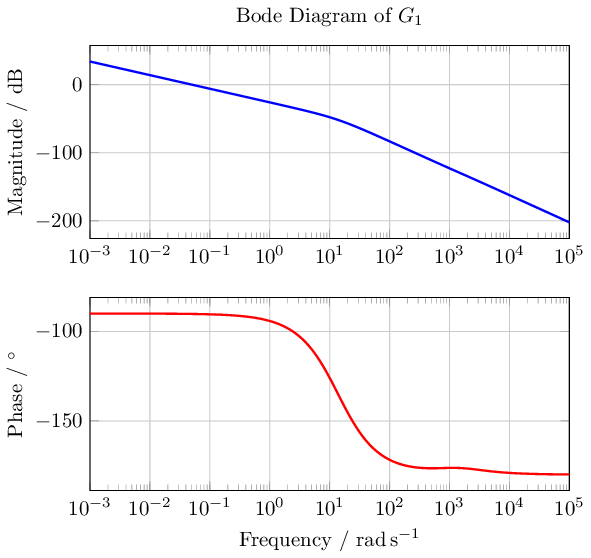 Bode diagram of the cart movement transfer function.
 -
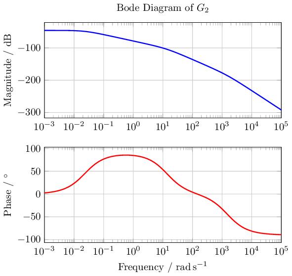 Bode diagram of the pendulums rotation transfer function.

