Ocs package
OCS : Octave Circuit Simulator
History and Motivation
OCS was developed during the CoMSON (Coupled Multiscale Simulation and Optimization) project which involved several universities but also several industrial partners.
Each of the industrial partners at the time was using its own circuit simulation software and each software had different file formats for circuit netlists.
Given the purposes of the project and the composition of the consortium the main design objectives for OCS where
- provide a format for "element evaluators" independent of time-stepping algorithms
- provide a "hierarchical" data structure where elements could be composed themselves of lumped-element networks
- allow coupling of lumped-element networks (0D) and 1D/2D/3D device models
- use an intermediate/interchange file format so that none of the formats in use by the industrial partners would be favoured over the others
- be written in an interpreted language for quick prototyping and easy maintainance
- be Free Software
Problem Formulation
The circuit description in OCS is based on (a variant of) modified nodal analysis (MNA) model for lumped-element networks. It is easy to verify that the common charge/flux-based MNA model is a special case of the model presented below.
We consider a circuit with M elements and N nodes, the core of the MNA model is a set of N equations of the form
where denotes the current from the node n due to element m.
The equations above are the Kirchhoff current law (KCL) for each of the electrical nodes of the network.
The currents can be expressed in terms of the node voltages and the internal variables
Notice that the variables only appear in the equations defining the fluxes relative to the m-th element, for this reason they are sometimes referred to as internal variables of the m-th element.
The full MNA model is finally obtained by substituting the current definitions in the KCL and complementing it with a suitable number of constitutive relations for the internal variables of each element
Notice that the assumption that only time derivatives of internal variables appear above and that terms involving such derivatives are linear does not impose restrictions on the applicability of the model.
Data Structure
A circuit is represented in OCS by a struct variable with the fields listed below
| Code: OCS structure format |
cir_struct =
{
  LCR:  struct      % the fields of LCR are shown below
  NLC:  struct      % NLC has the same fields as LCR
  namesn: matrix    % numbers of vars that are assigned a name in and.nms
  namess: cell      % the names corresponding to the vars above
  totextvar: scalar % the total number of external variables
  totintvar: scalar % the total number of internal variables
}

outstruct.LCR =
{
  1x2 struct array containing the fields: % array has one element per block

    func     % name of the sbn file corresponding to each block
    section  % string parameter to be passed to the sbn files
    nextvar  % number of external variables for each element of the block
    vnmatrix % numbers of the external variables of each element
    nintvar  % number of internal variables for each element of the block
    osintvar % number of the first internal variable
    npar     % number of parameters
    nparnames% number of parameter names
    nrows    % number of rows in the block
    parnames % list of parameter names
    pvmatrix % list of parameter values for each element

}
|
File Formats
There are several ways of setting up the data structure for an OCS simulation. The first approach is to just assign the fields of the data structure via Octave commands, otherwise one can parse an ascii file written in (a subste of) SPICE netlist language or in OCS's own netlist specification language called IFF (Interchange File Format)
IFF netlists
The name IFF stands for "Intermediate File Format" or "Interchange File Format" it represents an ASCII file format for describing coupled electrical circuits, devices and systems. The IFF syntx described here is version 0.1b1.
A circuit description is comprised of a set of files of three different types:
- 1 CIR (Circuit) file: an ASCII text file with filename <circuitname>.cir
- 1 NMS (Names) file: an ASCII text file with filename <circuitname>.nms
- N >= 1 SBN (Subnet) files: a set of M-functions or DLD-functions following the template described below.
SBN files are not necessarily specific to one circuit and can be grouped in libraries as long as the directory containing the library is added to the path when the IFF parser is run.
CIR file
The CIR file is divided into two sections describing the linear time–independent (LCR = linear circuit) and the non–linear and/or time–dependent (NLC = non–linear circuit) partitions of the circuit respectively. The syntax for the LCR and NLC section is identical. NLC can also contain linear elements, in fact the whole circuit could be described only by the NLC section but this could result in the evaluator unnecessarily recomputing local matrices for linear time–independent elements The content of CIR files is organized as follows:
| Code: CIR file format |
 cir    := header nlc separator lcr separator ;
 header := '%' version_id '$\nl$'
           comment* ;
 comment:= '%' text '$\nl$' ;
 nlc    := block* ;
 block  := blockcomment? blockheader pv_matrix vnum_matrix  ;
 block_comment := '%' text '$\nl$' ;
 block_header  := func section n_extvar n_par '$\nl$'
                  n_rows n_parnames '$\nl$'
                  par_name*;
 section      :=  string ;
 n_extvar     :=  number ;
 n_par        :=  number ;
 n_rows       :=  number ;
 n_parnames   :=  number ;
 par_name     :=  string ;
 pv_matrix    :=  matrix ;
 vnum_matrix  :=  matrix ;
 matrix    :=  number+ ;
 separator := 'END $\nl$' ;
 lcr       :=  block* ;
|
where
- "version_id" is a string identifying the version on IFF in which the file is encoded
- "\n" is the new-line character string that represents anything that the Octave command "s=fscanf(file,%s)" would parse as a string i.e. any sequence of chars without white-space
- "text" is any sequence of chars without a \n, this differs from string because it can contain white–space number represents anything that the Octave command "s=fscanf(file,%g)" would parse as a number
- "func" is the name of a function to evaluate the elements described in the block
- "n_extvar" Is the number of external variables for the elements of a block
- "n_par" Is the number of parameters for the elements of a block
- "n_rows" Is the number of elements in a block
- n_parnames" Is the number of parameter names for the elements of a block, it corresponds to the number of par name entries. If "n_parnames" is 0 the line with the "par_names" is missing.
- "pv_matrix" Is a list of n_rows x n_par numbers separated by any character the Octave command "s=fscanf(file,%g)" would consider whitespace (including "\n"). Every row (a set of n par contiguous entries) in "pv_matrix" refers to an element of the circuit. The "n_par" numbers in a row represent the values of the parameters to be passed to the function that evaluates that element.
- "vnum_matrix" Is a list of "n_rows" x "n_extvar" numbers separated by any character the Octave command "s=fscanf(file,%g)" would consider white-space (including \n). Every row (a set of "n_extvar" contiguous entries) in "vnum_matrix" refers to an element of the circuit. The "n_extvar" numbers in the row represent the global numbering of the element external variables.
NMS files
NMS files are meant to contain the names of the circuit variables, the format of NMS is just a list of variable names one on each row preceded by the variable number:
| Code: CIR file format |
nms := version id ’\n’ comment∗ line∗ ; line := var number var name ;
var number := number ;
var name := string ;
|
the variable are ordered as follows:
- first all external variables of all elements in the order given by the global numbering of external variables as explicitly written in the CIR files
- then the internal variables of the elements in the same order as the corresponding elements appear in the CIR file ( internal variables of non-linear elements first, then those of linear elements)
Notice that the number of internal variables of each element is not included in the IFF files. This is because elements with a number of internal variables that is huge, that depends on the value of some parameter, or even that changes in time (for example distributed elements treated with a FEM with adaptive meshing, a large linear sub- circuit that is reduce via MOR...) and therefore it is more convenient to compute the number of internal variables when initializing the system.
SBN files
SBN files are Octave functions, implemented as M-scripts or as DLD functions, with the following signature
| Code: Model evaluator file for simple MOSFET models |
function [a, b, c] =...
func (string , pvmatrix(i ,:) , extvar , intvar , t)
|
i.e. it should get as inputs:
- the string entry of the "block_header"
- one row of the "pv_matrix" entry of the "block"
- the current values of all internal and external variables
- the current time
and it should produce as outputs three matrices:
where "n_intvar" is the number of internal variables that can be assembled in the complete system matrices.
SPICE netlists
SPICE .spc netlists are parsed via the function "prs_spice", which currently supports the set of "Element Cards" shown below with their instantiating syntax.
| Code: Model evaluator file for simple MOSFET models |
 - Capacitors:
               Cname n+ n- cvalue

        - Diodes:
               Cname anode knode modelname <parameters>

        - MOS:
               Mname gnode dnode snode bnode modelname <parameters>

          N.B.: one instance of a MOS element MUST be preceeded
          (everywhere in the file) by the declaration of the related
          model.  For instance:
               .MODEL mynmos NMOS( k=1e-4 Vth=0.1 rd=1e6)
               M2 Vgate 0 Vdrain 0 mynmos

        - Resistors:
               Rname n+ n- rvalue

        - Voltage sources:
               Vname n+ n- <dcvalue> <transvalue>

          Transvalue specifies a transient voltage source
               SIN(VO  VA  FREQ TD  THETA)
          where:
             * VO (offset)
             * VA (amplitude)
             * FREQ (frequency)
             * TD (delay)
             * THETA (damping factor)

             * 0 to TD: V0
             * TD to TSTOP: VO +
               VA*exp(-(time-TD)*THETA)*sine(twopi*FREQ*(time+TD))

          Currently the damping factor has no effect.

          Pulse
               PULSE(V1 V2 TD TR  TF  PW  PER)

          parameters meaning
             * V1 (initial value)
             * V2 (pulsed value)
             * TD (delay time)
             * TR (rise time)
             * TF (fall time)
             * PW (pulse width)
             * PER (period)

          Currently rise and fall time are not implemented yet.

        - .MODEL cards Defines a model for semiconductor devices

               .MODEL MNAME TYPE(PNAME1=PVAL1 PNAME2=PVAL2 ... )

          TYPE can be:
             * NMOS N-channel MOSFET model
             * PMOS P-channel MOSFET model
             * D diode model

          The parameter "LEVEL" is currently assigned to the field
          "section" in the call of the element functions by the solver.
          Currently supported values for the parameter LEVEL for NMOS
          and PMOS are:
             * simple
             * lincap
          (see documentation of function Mdiode).

          Currently supported values for the parameter LEVEL for D are:
             * simple
          (see documentation of functions Mnmosfet and Mpmosfet).
|
Tutorials
A CMOS AND GATE
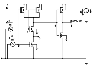
Here we show how to set up the simulation of the CMOS AND gate in the figure. The circuit has
- 9 Elements
- 6 MOSFETs (3 n-type + 3 p-type)
- 3 Voltage sources
For the n-type MOSFETs we use a very simple algebraic model defined by the following code
| Code: Model evaluator file for simple MOSFET models |
function [a,b,c] = Mnmosfet (string, parameters, parameternames, extvar, intvar, t)

  switch string

    case 'simple',

      rd = 1e6;

      for ii=1:length(parameternames)
        eval([parameternames{ii} "=",...
              num2str(parameters(ii)) " ;"])
      endfor

      vg   = extvar(1);
      vs   = extvar(2);
      vd   = extvar(3);
      vb   = extvar(4);

      vgs  = vg-vs;
      vds  = vd-vs;

      if (vgs < Vth)


        gm = 0;
        gd = 1/rd;
        id = vds*gd;

      elseif ((vgs-Vth)>=(vds))&(vds>=0)

        id = k*((vgs-Vth)*vds-(vds^2)/2)+vds/rd;
        gm = k*vds;
        gd = k*(vgs-Vth-vds)+1/rd;

      elseif ((vgs-Vth)>=(vds))&(vds<0)

        gm = 0;
        gd = 1/rd;
        id = vds*gd;

      else # (i.e. if 0 <= vgs-vth <= vds)

        id = k*(vgs-Vth)^2/2+vds/rd;
        gm = k*(vgs-Vth);
        gd = 1/rd;

      endif

      a = zeros(4);

      b = [ 0     0         0   0;
           -gm   (gm+gd)   -gd  0;
            gm  -(gm+gd)    gd  0;
            0     0         0   0];

      c = [0 -id id 0]';
      break;

    otherwise

      error(["Mnmosfet: unknown option " string]);

  endswitch

endfunction
|
The model for the p-type devices is entirely analogous.
Below we show three methods for constructing the circuit data structure
Once the circuit data structure is loaded the simulation can be started by the following commands
| Code: Run the AND gate simulation |
x         = [.5 .5 .33 .66 .5 1 0 0 1 ]';
t         = linspace (0, .5, 100);
pltvars   = {"Va", "Vb", "Va_and_b"};
dmp       = .2;
tol       = 1e-15;
maxit     = 100;
out       = tst_backward_euler (outstruct, x, t, tol, maxit, pltvars);
|
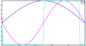
Click on the figure to the right to see the simulation results
Build the AND GATE structure directly
| Code: Build the AND GATE structure via an Octave script |
## NLC

# n-type
outstruct.NLC(1).func = "Mnmosfet";
outstruct.NLC(1).section = "simple";
outstruct.NLC(1).nextvar = 4;
outstruct.NLC(1).npar = 3;
outstruct.NLC(1).nparnames = 3;
outstruct.NLC(1).parnames = { "k", "Vth", "rd"};

outstruct.NLC(1).pvmatrix = [1.0000e-04   1.0000e-01   1.0000e+07
                             1.0000e-04   1.0000e-01   1.0000e+07
                             1.0000e-04   1.0000e-01   1.0000e+07];

outstruct.NLC(1).vnmatrix = [1   3   4   0
                             2   0   3   0
                             4   0   5   0];

outstruct.NLC(1).nintvar = [0 0 0];
outstruct.NLC(1).osintvar = [0 0 0];


# p-type
outstruct.NLC(2).func = "Mpmosfet";
outstruct.NLC(2).section = "simple";
outstruct.NLC(2).nextvar = 4;
outstruct.NLC(2).npar = 3;
outstruct.NLC(2).nparnames = 3;
outstruct.NLC(2).parnames = { "k", "Vth", "rd"};
outstruct.NLC(2).pvmatrix = [-1.0000e-04  -1.0000e-01   1.0000e+07
                             -1.0000e-04  -1.0000e-01   1.0000e+07
                             -1.0000e-04  -1.0000e-01   1.0000e+07];
outstruct.NLC(2).vnmatrix =  [ 1   6   4   6
                               2   6   4   6
                               4   6   5   6];

outstruct.NLC(2).nintvar = [0 0 0];
outstruct.NLC(2).osintvar = [0 0 0];

# Va and Vb

outstruct.NLC(3).func = "Mvoltagesources";
outstruct.NLC(3).section = "sinwave";
outstruct.NLC(3).nextvar = 2;
outstruct.NLC(3).npar = 4;
outstruct.NLC(3).nparnames = 4;
outstruct.NLC(3).parnames = {"Ampl", "f", "delay", "shift"};
outstruct.NLC(3).pvmatrix = [0.50000   1.00000   0.00000   0.50000
                             0.50000   2.00000   0.25000   0.50000];
outstruct.NLC(3).vnmatrix = [ 1   0
                              2   0];
outstruct.NLC(3).nintvar = [1 1];
outstruct.NLC(3).osintvar = [0 0];

## LCR

# Vdd
outstruct.LCR(1).func = "Mvoltagesources";
outstruct.LCR(1).section = "DC";
outstruct.LCR(1).nextvar = 2;
outstruct.LCR(1).npar = 1;
outstruct.LCR(1).nparnames = 1;
outstruct.LCR(1).parnames = {"V"};
outstruct.LCR(1).pvmatrix = 1;
outstruct.LCR(1).vnmatrix = [6 0];
outstruct.LCR(1).nintvar = 1;
outstruct.LCR(1).osintvar = 2;

##

outstruct.namesn = [1   2   5   6   7   8   9];
outstruct.namess = {"Va", "Vb", "Va_and_b", "Vdd", "I1", "I2", "I3"};
outstruct.totextvar =  6;
outstruct.totintvar =  3;
|
Build the AND gate circuit structure parsing an IFF netlist
To parse an IFF format netlist of the CMOS AND gate we can use the following command
| Code: Load the AND circuit structure parsing an IFF netlist |
outstruct = prs_iff ("and");
|
The IFF netlist consists of the .cir file named "and.cir" shown below
| Code: IFF netlist for the AND gate (.cir file) |
% 0.1b1
% A Simple CMOS AND GATE
%
% N-Mosfets
% There are 3 N-Mosfets
Mnmosfet simple 4 3
3 3
k          Vth		rd
1e-4       0.1		1e7
1e-4       0.1		1e7
1e-4       0.1		1e7
1 3 4 0
2 0 3 0
4 0 5 0
%
% P-Mosfets
Mpmosfet simple 4 3
3 3
k           Vth		rd
-1e-4       -0.1	1e7
-1e-4       -0.1	1e7
-1e-4       -0.1	1e7
1 6 4 6
2 6 4 6
4 6 5 6
%
% Input voltage sources
Mvoltagesources sinwave 2 4
2 4
Ampl      f       delay     shift
0.5       1       0.0       0.5
0.5       2       0.25      0.5
1 0
2 0
END
%
% Power supply
Mvoltagesources DC  2 1
1 1
V
1
6 0
END
|
and of the .nms file named "and.nms shown below
| Code: IFF netlist for the AND gate (.nms file) |
% 0.1b1
1 Va
2 Vb
5 Va_and_b
6 Vdd
7 I1
8 I2
9 I3
|
Build the AND gate circuit structure parsing a .spc file
| Code: Load the AND circuit structure parsing a .spc file |
outstruct = prs_spice ("and");
|
| Code: The .spc file for the CMOS AND gate |
* AND (simple Algebraic MOS-FET model)

.MODEL mynmos NMOS(LEVEL=simple k=2.94e-05   Vth=0.08	rd=.957e7)
.MODEL mypmos PMOS( k=-2.94e-05   Vth=-0.08	rd=.957e7)

M1 Va 3  4        0 mynmos
M2 Vb 0  3        0 mynmos
* nside of the inverter
M3 4  0  Va_and_b 0 mynmos

M4 Va Vdd 4        Vdd  mypmos
M5 Vb Vdd 4        Vdd  mypmos

* pside of the inverter
M6 4  Vdd Va_and_b Vdd  mypmos

V1  Va 0 SIN(0.5 0.5 1 0 0)
V2  Vb 0 SIN(0.5 0.5 2 0.25 0)
V3  Vdd 0 1

.END
|
A circuit with a linear VCVS
To parse an IFF format netlist of the VCVS circuit we can use the following command
| Code: Load the VCVS circuit structure parsing an IFF netlist |
outstruct = prs_iff ("vcvs");
|
The IFF netlist consists of the .cir file named "vcvs.cir" shown below
| Code: IFF netlist for the VCVS circuit (.cir file) |
%0.1b1
% A Simple linear VCVS example
% Input voltage sources
Mvoltagesources sinwave 2 4
1 4
Ampl      f       delay     shift
1         1       0.0       0.0
1 0
END
% VCVS
Mvcvs LIN 4 1
1 1
Gain
5.0
2 0 1 0
% Resistor
Mresistors LIN  2 1
1 1
R
1
1 2
END
|
and of the .nms file named "and.nms shown below
| Code: IFF netlist for the VCVS circuit (.nms file) |
% 0.1b1
1 V_controller
2 V_controlled
|
The implementation for the VCVS with linear gain is shown below
| Code: Model evaluator file for simple VCVS model |
function [a,b,c] = Mvcvs (string, parameters, parameternames, extvar,
                          intvar, t)

  if isempty(intvar)
    intvar = 0;
  endif

  switch string
      ##LCR part
    case "LIN"
      for ii=1:length(parameternames)
	eval([parameternames{ii} "=" num2str(parameters(ii)) ";"])
      endfor

      j = intvar (1);
      Vin = extvar (3) - extvar (4);
      V = Vin * Gain;

      a = zeros (5);
      b = [0  0   0     0     1;
           0  0   0     0    -1;
           0  0   0     0     0;
           0  0   0     0     0;
           1 -1  -Gain  Gain  0];

      c = [0 0 0 0 0];
      break

    otherwise
      error (["unknown section:" string])
  endswitch

endfunction
|
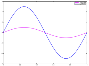
To run a simulation with this circuit use the following commands:
| Code: Run a simple transient simulation with the VCVS circuit |
>> x = [0 0 0 0]';
>> t = linspace(0,1,50);
>> [out, niter] = tst_backward_euler (outstruct, x, t, 1e-6, 100, pltvars, [0 1]);
|
Creating a model for a memristor device
To demonstrate how to write a model evaluator file (SBN file), we will discuss the simplest memristor model shown in this paper by KaKiLa et al.:
Carbajal, J. P. et al. Memristor models for machine learning. Neural Computation, 27(3), 2015. doi:10.1162/NECO_a_00694
The device model is presented in the original paper as
The first thing to do is to change the model from impedance to admittance form and write the constitutive relation for the internal variable in an "implicit form"
It is then useful to compute the derivatives for the current and for the constitutive relation
Next we define external variables (pin voltages) for the device and coupling variables (pin currents)
 N.B. the convention in existing device models is that pin currents are
      assumed to be entering the device
Now define the local state vector
and the local equations
and finally define the local matrices for the memristor element
The resulting model implementation is the following
| Code: memristor model implementation |
function [a,b,c] = Mmemristors (string, parameters, parameternames,
                                extvar, intvar, t)

  if isempty(intvar)
    intvar = 0;
  endif

  switch string
    case "STRUKOV"
      ## NLC part
      for ii=1:length(parameternames)
	eval([parameternames{ii} "=" num2str(parameters(ii)) ";"])
      endfor

      v1 = extvar(1);
      v2 = extvar(2);
      x  = intvar(1);

      if (x <= 0)
        H = RH;
        Hp = 0;
      elseif (x > 0 && x < 1)
        H = RH - (RH - RL) * x;
        Hp = - (RH - RL);
      else
        H = RL;
        Hp = 0;
      endif

      I  = (v1-v2) / H;
      i1 = I;
      i2 = -I;

      dIdx = - Hp / H^2;
      dIdV = 1 / H;

      a = zeros (3);
      a(3, 3) = 1/ MU;

      b = [dIdV  -dIdV dIdx;
           -dIdV dIdV  -dIdx;
           -dIdV dIdV  -dIdx];

      c = [i1 i2 i2]';

      break;

    otherwise
      error (["unknown section:" string])
  endswitch

endfunction
|
As an example let's run a simulation by applying a sinusoidal signal with varying frequency
| Code: memristor model implementation |
t = linspace (0, 1, 100);
y = [(sin (2 * pi * t * 1.5)), (sin (2 * pi * t * 4))(2:end)];
t = [t, (linspace (1, 2, 100))(2:end)];
pwl = [t; y](:).';

c1.LCR = [];
c1.totextvar = 1;

c1.NLC(1).("func") = "Mvoltagesources";
c1.NLC(1).("section") = "pwl";
c1.NLC(1).("nextvar") = 2;
c1.NLC(1).("npar") = 398;
c1.NLC(1).("nrows") = 1;
c1.NLC(1).("nparnames") = 0;
c1.NLC(1).("parnames") = {};
c1.NLC(1).("pvmatrix") = pwl;
c1.NLC(1).("vnmatrix") = [1 0];
c1.NLC(1).("nintvar") = 1;
c1.NLC(1).("osintvar") = 0;

c1.NLC(2).("func") = "Mmemristors";
c1.NLC(2).("section") =  "STRUKOV";
c1.NLC(2).("nextvar") =  2;
c1.NLC(2).("npar") =  3;

c1.totintvar = 2;
c1.namesn = [1   2   3];

c1.NLC(2).("nrows") =  1;
c1.NLC(2).("nparnames") =  3;
c1.NLC(2).("parnames") =  {"MU", "RH", "RL"};
c1.NLC(2).("pvmatrix") =  [1.8e3 1e3 1];
c1.NLC(2).("vnmatrix") =  [1 0];

c1.NLC(2).("nintvar") =  1;
c1.NLC(2).("osintvar") =  1;

c1.namess = {"voltage", "current", "x"};
start = [0 0 0.1];

%% c = prs_iff ("memristor_example");
out = tst_backward_euler (c1, start.', t, 1e-2, 300, {'voltage', 'current'});

plot (out(1, 1:100), out (2, 1:100), 'r',
      out(1, 101:end), out(2, 101:end), 'k')

legend ("frequency 1 Hz", "frequency 4 Hz")
|
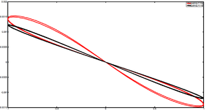
The results are shown in the figure to the right.
Dependencies
Odepkg
Ocs depends on odepkg that is not anymore part of the Octave Forge project. However, odepkg still works as of 2020, and instructions to install it are available in this wiki.


![{\displaystyle \sum _{{m}=1}^{M}\left[\ A_{mn}{\dot {r}}_{m}+J_{mn}\left({e},{r}_{m}\right)\right]=0\qquad {\begin{array}{l}{n}=1,\,\ldots \,,N\end{array}}}](https://wikimedia.org/api/rest_v1/media/math/render/svg/629f66da6bff3b311b18cea5ae8ba9adccd53f6a)


![{\displaystyle z=\left[{\begin{array}{l}v^{+}\\v^{-}\\x\end{array}}\right]}](https://wikimedia.org/api/rest_v1/media/math/render/svg/9179275b223f171b5a0eca66c656e31a5de62b00)

![{\displaystyle a=\left[{\begin{array}{c c c}0&0&0\\0&0&0\\0&0&{\dfrac {1}{\mu }}\end{array}}\right]}](https://wikimedia.org/api/rest_v1/media/math/render/svg/f948dd0301b4918bc7818e779bc9a087d3ea2cbf)
![{\displaystyle c(z)=\left[{\begin{array}{c}{\dfrac {V}{H}}\\[2mm]-{\dfrac {V}{H}}\end{array}}\right]}](https://wikimedia.org/api/rest_v1/media/math/render/svg/b46fd24bffcbe0dd43bbcf4c555c0131b3ba1665)
![{\displaystyle b(z)={\dfrac {\partial c}{\partial z}}=\left[{\begin{array}{c c c}{\dfrac {\partial I}{\partial V}}&-{\dfrac {\partial I}{\partial V}}&{\dfrac {\partial I}{\partial x}}\\[2mm]-{\dfrac {\partial I}{\partial V}}&+{\dfrac {\partial I}{\partial V}}&-{\dfrac {\partial I}{\partial x}}\\[2mm]-{\dfrac {\partial I}{\partial V}}&+{\dfrac {\partial I}{\partial V}}&-{\dfrac {\partial I}{\partial x}}\\[2mm]\end{array}}\right]}](https://wikimedia.org/api/rest_v1/media/math/render/svg/1cdf1be643fa5b756e236518d3609e9b42f2b04c)
