TISEAN package

Porting TISEAN

This section will focus on demonstrating the capabilities of the TISEAN package. The previous information about the porting procedure has been moved here.

Current ideas and future plans are available on a board loacated here

Tutorials

These tutorials are based on examples, tutorials and the articles located on the TISEAN website:
http://www.mpipks-dresden.mpg.de/~tisean/Tisean_3.0.1/.
This tutorial will utilize the following dataset:

• amplitude.dat

Please download it as the tutorial will reference it.

False Nearest Neighbors

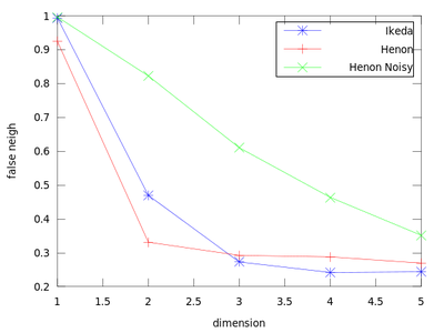
This function uses a method to determine the minimum sufficient embedding dimension. It is based on the False Nearest Neighbors section of the TISEAN documentation. As a demonstration we will create a plot that contains an Ikeda Map, a Henon Map and a Henon Map corrupted by 10% of Gaussian noise.

Code: Analyzing false nearest neighbors

# Create maps ikd = ikeda (10000); hen = henon (10000); hen_noisy = hen + std (hen) * 0.02 .* (-6 + sum (rand ([size(hen), 12]), 3)); # Create and plot false nearest neighbors [dim_ikd, frac_ikd] = false_nearest (ikd(:,1)); [dim_hen, frac_hen] = false_nearest (hen(:,1)); [dim_hen_noisy, frac_hen_noisy] = false_nearest (hen_noisy(:,1)); plot (dim_ikd, frac_ikd, '-b*;Ikeda;',... dim_hen, frac_hen, '-r+;Henon;',... dim_hen_noisy, frac_hen_noisy, '-gx;Henon Noisy;');

The dim_* variables hold the dimension (so here 1:5), and frac_* contain the fraction of false nearest neighbors. From this chart we can obtain the sufficient embedding dimension for each system. For a Henon Map m = 2 is sufficient, but for an Ikeda map it is better to use m = 3.

Finding Unstable Periodic Orbits

Here I will demonstrate how to find unstable periodic orbits. This section is based on the TISEAN documentation chapter Finding unstable periodic orbits. We will start by finding these orbits using function upo.

Code: Finding unstable periodic orbits

# Create maps hen = henon (1000); hen = hen + std (hen) * 0.02 .* (-6 + sum (rand ([size(hen), 12]), 3)); # Find orbits [lengths, data] = upo(hen(:,1), 2, 'p',6,'v',0.1, 'n', 100);

The vector lengths contains the size of each of the found orbits and data contains their coordinates. To obtain delay coordinates and plot these orbits onto the original data we will use upoembed.

Code: Plotting unstable periodic orbits

# Create delay coordinates for the orbits and data up = upoembed (lengths, data, 1); delay_hen = delay (hen(:,1)); # Plot all of the data plot (delay_hen(:,1), delay_hen(:,2), 'r.;Noisy Henon;','markersize',2,... up{4}(:,1), up{4}(:,2),'gx;Fixed Point;','markersize',20,'linewidth',1, ... up{3}(:,1), up{3}(:,2),'b+;Period 2;','markersize',20,'linewidth',1, ... up{2}(:,1), up{2}(:,2),'ms;Period 6;','markersize',20,'linewidth',1, ... up{1}(:,1), up{1}(:,2),'cs;Period 6;','markersize',20,'linewidth',1);

The plotting options are passed to make the orbits more visible.

Nonlinear Prediction

In this section we will demonstrate some functions from the 'Nonlinear Prediction' chapter of the TISEAN documentation (located here). For now this section will only demonstrate functions that are connected to the Simple Nonlinear Prediction section.
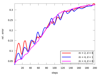
There are three functions in this section: lzo_test, lzo_gm and lzo_run. The first is used to estimate the forecast error for a set of chosen parameters, the second gives some global information about the fit and the third produces predicted points. Let us start with the first one (before starting this example remember to download 'amplitude.dat' from above and start Octave in the directory that contains it). The pairs of parameters (m,d) where chosen after the TISEAN documentation.

Code: Analyzing forecast errors for various parameters

# Load data load amplitude.dat # Create different forecast error results steps = 200; res1 = lzo_test (amplitude(1:end-200), 'm', 2, 'd', 6, 's', steps); res2 = lzo_test (amplitude(1:end-200), 'm', 3, 'd', 6, 's', steps); res3 = lzo_test (amplitude(1:end-200), 'm', 4, 'd', 1, 's', steps); res4 = lzo_test (amplitude(1:end-200), 'm', 4, 'd', 6, 's', steps); plot (res1(:,1), res1(:,2), 'r;m = 2, d = 6;', ... res2(:,1), res2(:,2), 'g;m = 3, d = 6;',... res3(:,1), res3(:,2), 'b;m = 4, d = 1;',... res4(:,1), res4(:,2), 'm;m = 4, d = 6;');

It seems that the last pair (m = 4, d = 6) is suitable. We will use it to determine the the best neighborhood to use when generating future points.

Code: Determining the best neighborhood size using lzo_gm

gm = lzo_gm (amplitude(1:end-200), 'm', 4, 'd', 6, 's', steps, 'rhigh', 20);

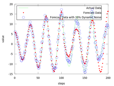
After analyzing gm it is easy to observe that the least error is for the first neighborhood size of gm which is equal to 0.49148. We will use it to produce the prediction vectors. Only the first 4800 datapoints from amplitude are used in order to compare the predicted values with the actual ones for the last 200 points.

Code: Creating forecast points

steps = 200; forecast = lzo_run (amplitude(1:end-200), 'm', 4, 'd', 6, 'r', 0.49148, 'l', steps); forecast_noisy = lzo_run (amplitude(1:end-200), 'm', 4, 'd', 6, 'r', 0.49148, ... 'dnoise', 10, 'l', steps); plot (amplitude(end-199:end), 'g;Actual Data;', ... forecast, 'r.;Forecast Data;',... forecast_noisy, 'bo;Forecast Data with 10% Dynamic Noise;');

The difference between finding the proper r and not finding it can be very small.
The produced data is the best local zeroth order fit on the amplitude.dat for (m = 4, d = 6).

Nonlinear Noise Reduction

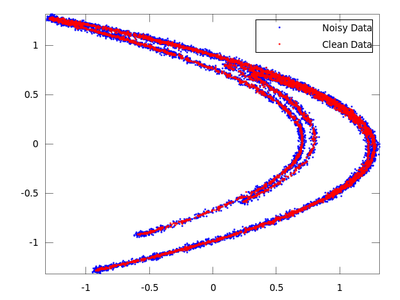
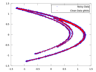
This tutorial show different methods of the 'Nonlinear Noise Reduction' section of the TISEAN documentation (located here). It shows the use of simple nonlinear noise reduction (function lazy) and locally projective nonlinear noise reduction (function ghkss). To start let's create noisy data to work with.

Code: Creating a noisy henon map

hen = henon (10000); hen = hen(:,1); # We only need the first column hen_noisy = hen + std (hen) * 0.02 .* (-6 + sum (rand ([size(hen), 12]), 3));

This created a Henon map contaminated by 2% Gaussian noise à la TISEAN. In the tutorials and exercises on the TISEAN website this would be equivalent to calling makenoise -%2 on the Henon map.
Next we will reduce the noise using simple nonlinear noise reduction lazy.

Code: Simple nonlinear noise reduction

clean = lazy (hen_noisy,7,-0.06,3); # Create delay vectors for both the clean and noisy data delay_clean = delay (clean); delay_noisy = delay (hen_noisy); # Plot both on one chart plot (delay_noisy(:,1), delay_noisy(:,2), 'b.;Noisy Data;','markersize',3,... delay_clean(:,1), delay_clean(:,2), 'r.;Clean Data;','markersize',3)

On the chart created the red dots represent cleaned up data. It is much closer to the original than the noisy blue set.
Now we will do the same with ghkss.

Code: Locally projective nonlinear noise reduction

clean = ghkss (hen,'m',7,'q',2,'r',0.05,'k',20,'i',2);

The rest of the code is the same as the code used in the lazy example.
Once both results are compared it is quite obvious that for this particular example ghkss is superior to lazy. The TISEAN documentation points out that this is not always the case.

External links

• Bitbucket repository where the porting is taking place.
• TISEAN package website where the package is described along with references to literature, tutorials and manuals.