|
|
| Line 1: |
Line 1: |
| == Porting TISEAN == | | == Porting TISEAN == |
|
| |
|
| This section will focus on demonstrating how the package is to be ported and what is the current state of that process. | | This section which focuses on demonstrating how the package is to be ported and what is the current state of that process is located in [[TISEAN_package:Procedure]]. |
| | |
| === Process ===
| |
| | |
| This section describes the process employed during porting TISEAN package into an Octave Package. This project was started as part of the Google Summer of Code 2015.
| |
| | |
| To aid in understanding the task there are some charts.
| |
| | |
| The first chart depicts what to do with each function in the function table. I mainly focuses on those functions that might already implemented in Octave.
| |
| | |
| [[File:Work_flow_TISEAN.png|400px|center]]
| |
| | |
| The chart below depicts how to decide which type of port should be utilized.
| |
| | |
| [[File:Porting_Programs_TISEAN.png|400px|center]] | |
| | |
| Both of those charts can be combined into a large one that shows all of the work together.
| |
| | |
| [[File:Flow_Together_TISEAN.png|400px|center]]
| |
| === Table of functions and progress ===
| |
| In reference to the TISEAN library alphabetical order of programs which is located [http://www.mpipks-dresden.mpg.de/~tisean/Tisean_3.0.1/docs/alphabetical.html here].
| |
| | |
| The choice whether a program exist in Octave is based only on comparing package/octave documentation with the TISEAN documentation. As of now I have not compared any code, nor checked if any sample data gives the same results from both functions (the octave ones and the TISEAN ones).
| |
| | |
| The legend to understand the table is as follows:
| |
| {| class="wikitable"
| |
| |-style="background: LightGreen"
| |
| |Green means the function is ported, tested or is not needed
| |
| |-style="background: LightSalmon"
| |
| |Red means the function was thought to have been similar but isn't
| |
| |-style="background: Yellow"
| |
| |Yellow means that the correlation between the TISEAN and Octave function needs to be verified
| |
| |-
| |
| |No color means that nothing about this function has been determined
| |
| |}
| |
| | |
| {| class="wikitable"
| |
| |-
| |
| ! Program Name !! Program Description !! Corresponding Octave Function !! Lanuguage of Origin !! How to port !! Status
| |
| |-
| |
| | arima-model || Fit and possibly iterate an ARIMA model || generalizes TSA arma functions || C || wrapped in C++/mfile/octfile code ||
| |
| |-
| |
| |ar-model || Fit and possibly iterate an Autoregessive model || 'aar' in TSA; see also: aarmam, adim, amarma, mvaar from TSA || C || wrapped in C++/mfile/octfile code ||
| |
| |-
| |
| |ar-run || Iterate an Autoregessive model || Same as above || FORTRAN || wrapped in C++/mfile/octfile code ||
| |
| |-style="background: LightGreen"
| |
| |av-d2 || Simply smooth output of d2 || Can be implemented with filter in core || C || ||
| |
| |-style="background: LightGreen"
| |
| |boxcount || Renyi Entopies of Qth order || None in GNU Octave (maybe in info-theory but it is not worth the pain) || C || wrapped in C++/mfile/octfile code ||
| |
| |-style="background: LightGreen"
| |
| |c1 || Fixed mass estimation of D1 || None in GNU Octave || FORTRAN || wrapped in C++/mfile/octfile code ||
| |
| |-style="background: LightGreen"
| |
| |c2d || Get local slopes from correlation integral || None in GNU Octave || FORTRAN || wrapped in C++/mfile/octfile code ||
| |
| |-style="background: LightGreen"
| |
| |c2g || Gaussian kernel of C2 || None in GNU Octave || FORTRAN || wrapped in C++/mfile/octfile code ||
| |
| |-style="background: LightGreen"
| |
| |c2t || Takens estimator of D2 || None in GNU Octave || FORTRAN || wrapped in C++/mfile/octfile code ||
| |
| |-style="background: LightGreen"
| |
| |choose || Choose rows and/or columns from a data file || Does not need to be ported || FORTRAN || ----- || Not Needed
| |
| |-style="background: LightGreen"
| |
| |compare || Compares two data sets || Does not need to be ported || FORTRAN || ------ || Not Needed
| |
| |-style="background: LightGreen"
| |
| |corr, autocorr || Autocorrelation function || xcorr in signal || corr -C, autocorr (faster according to documentation) - FORTRAN || ------- || Different usage, same result
| |
| |-style="background: LightGreen"
| |
| |d2 || Correlation dimension d2 || None in GNU Octave || C || wrapped in C++/mfile/octfile code ||
| |
| |-style="background: LightGreen"
| |
| |delay || Creates delay embedding || None in GNU Octave (easy to implement in Octave but not worth the effort) || C || wrapped in C++/mfile/octfile code || Ported&Tested
| |
| |-style="background: LightGreen"
| |
| |endtoend || Determine end-to-end mismatch || None in GNU Octave || FORTRAN || wrapped in C++/mfile/octfile code || Ported&Tested
| |
| |-
| |
| |events || Interval/event conversion || None in GNU Octave || FORTRAN || To be reimplemented as m-file ||
| |
| |-style="background: LightSalmon"
| |
| |extrema || Determine the extrema of a time series || findpeaks in signal is *not* the same || C || ||
| |
| |-style="background: LightGreen"
| |
| |false_nearest || The false nearest neighbor algorithm || None in GNU Octave || C || wrapped in C++/mfile/octfile code || Ported&Tested
| |
| |-style="background: LightGreen"
| |
| |ghkss || Nonlinear noise reduction || None in GNU Octave || C || wrapped in C++/mfile/octfile code || Ported&Tested
| |
| |-style="background: LightGreen"
| |
| |henon || Create a Hénon time series || None in GNU Octave || FORTRAN || To be reimplemented as m-file || Ported&Checked
| |
| |-style="background: LightGreen"
| |
| |histogram || Creates histograms || hist in core || C || || Different usage, same result
| |
| |-style="background: LightGreen"
| |
| |ikeda || Create an Ikeda time series || None in GNU Octave || FORTRAN || To be reimplemented as mfile || Ported&Tested
| |
| |-
| |
| |intervals || Event/intervcal conversion || Might exist under different name || FORTRAN || To be reimplemented as mfile ||
| |
| |-style="background: LightGreen"
| |
| |lazy || Simple nonlinear noise reduction || None in GNU Octave || FORTRAN || wrapped in C++/mfile/octfile code || Ported&Tested
| |
| |-style="background: LightGreen"
| |
| |lfo-ar || Locally first order model vs. global AR model (old ll-ar) || None in GNU Octave || C || wrapped in C++/mfile/octfile code ||
| |
| |-style="background: LightGreen"
| |
| |lfo-run || Iterate a locally first order model (old nstep) || None in GNU Octave || C || wrapped in C++/mfile/octfile code ||
| |
| |-style="background: LightGreen"
| |
| |lfo-test || Test a locally first order model (old onestep) || None in GNU Octave || C || wrapped in C++/mfile/octfile code ||
| |
| |-style="background: Yellow"
| |
| |lorenz || Create a Lorenz time series || Can be implemented in GNU Octave using lsode or odepkg|| FORTRAN || mfile ||
| |
| |-
| |
| |low121 || Time domain low pass filter || There are lowpass filters in Octave: buttap, cheb1ap, cheb2ap, ellipap, sftrans, but I don't think they perform this task || C || Reimplement as mfile ||
| |
| |-style="background: LightGreen"
| |
| |lyap_k || Maximal Lyapunov exponent with the Kantz algorithm || None in GNU Octave || C || wrapped in C++/mfile/octfile code ||
| |
| |-style="background: LightGreen"
| |
| |lyap_r || Maximal Lyapunov exponent with the Rosenstein algorithm || None in GNU Octave || C || wrapped in C++/mfile/octfile code ||
| |
| |-style="background: LightGreen"
| |
| |lyap_spec || Full spectrum of Lyapunov exponents || None in GNU Octave || C || wrapped in C++/mfile/octfile code ||
| |
| |-style="background: LightGreen"
| |
| |lzo-gm || Locally zeroth order model vs. global mean || None in GNU Octave || C || wrapped in C++/mfile/octfile code || Ported&Tested
| |
| |-style="background: LightGreen"
| |
| |lzo-run || Iterate a locally zeroth order model || None in GNU Octave || C || wrapped in C++/mfile/octfile code || Ported&Tested
| |
| |-style="background: LightGreen"
| |
| |lzo-test || Test a locally zeroth order model (old zeroth) || None in GNU Octave || C || wrapped in C++/mfile/octfile code || Ported&Tested
| |
| |-
| |
| |makenoise || Produce noise || Rand exists || Should be implemented as mfile using Octave rand functions || wrapped in C++/mfile/octfile code ||
| |
| |-
| |
| |mem_spec || Power spectrum using the maximum entropy principle || None in GNU Octave || C || wrapped in C++/mfile/octfile code ||
| |
| |-style="background: LightGreen"
| |
| |mutual || Estimate the mutual information || None in GNU Octave || C || wrapped in C++/mfile/octfile code || Ported&Tested
| |
| |-style="background: Yellow"
| |
| |notch || Notch filter || pei_tseng_notch, needs to be verified || FORTRAN || wrapped in C++/mfile/octfile code ||
| |
| |-
| |
| |nstat_z || Nonstationarity testing via cross-prediction || None in GNU Octave || C ||wrapped in C++/mfile/octfile code ||
| |
| |-style="background: LightGreen"
| |
| |pca, pc || Principle component analysis || 'pcacov' if likely the equivalent; pricomp in statistics || pca - C, pc - FORTRAN || wrapped in C++/mfile/octfile code || Ported&Tested
| |
| |-style="background: LightGreen"
| |
| |poincare || Create Poincaré sections || None in GNU Octave || C || wrapped in C++/mfile/octfile code || Ported&Tested
| |
| |-style="background: LightSalmon"
| |
| |polyback || Fit a polynomial model (backward elimination) || polyfit, detrend, wpolyfit are not similar || C || wrapped in C++ || Porting needed
| |
| |-style="background: LightGreen"
| |
| |polynom || Fit a polynomial model || same as above || C || || Ported&Tested
| |
| |-style="background: LightSalmon"
| |
| |polynomp || Fit a polynomial model (reads terms to fit from file) || same as above || C || ||
| |
| |-style="background: LightSalmon"
| |
| |polypar || Creates parameter file for polynomp || same as above || C || ||
| |
| |-style="background: LightGreen"
| |
| |predict || Forecast discriminating statistics for surrogates || None in GNU Octave || FORTRAN || wrapped in C++/mfile/octfile code || Same as lzo_test; Not Needed
| |
| |-
| |
| |randomize || General constraint randomization (surrogates) || There are random function, but I don't think this one exists || FORTRAN || wrapped in C++/mfile/octfile code ||
| |
| |-
| |
| |randomize_spikeauto_exp_random || Surrogate data preserving event time autocorrelations || Same as above || FORTRAN || wrapped in C++/mfile/octfile code ||
| |
| |-
| |
| |randomize_spikespec_exp_event || Surrogate data preserving event time power spectrum || Same as above || FORTRAN || wrapped in C++/mfile/octfile code ||
| |
| |-style="background: LightGreen"
| |
| |rbf || Radial basis functions fit || None in GNU Octave || C || wrapped in C++/mfile/octfile code ||
| |
| |-
| |
| |recurr || Creates a recurrence plot || None in GNU Octave || C || wrapped in C++/mfile/octfile code ||
| |
| |-style="background: Yellow"
| |
| |resample || Resamples data || interp1 is similar but cannot specify the polynomial order except for some given || C || wrapped in C++/mfile/octfile code ||
| |
| |-style="background: LightGreen"
| |
| |rescale || Rescale data set || This is just multiplication by scalars || C || wrapped in C++/mfile/octfile code ||Not Needed
| |
| |-style="background: LightGreen"
| |
| |rms || Rescale data set and get mean, variance and data interval || This should be in Octave, cannot find... || FORTRNAN || wrapped in C++/mfile/octfile code || Not Needed
| |
| |-style="background: Yellow"
| |
| |sav_gol || Savitzky-Golay filter || sgolayfilt in signal || C || ||
| |
| |-style="background: LightGreen"
| |
| |spectrum || Power spectrum using FFT || abs (fft (;)) || FORTRAN || Rewrite as m-file || Ported&Tested
| |
| |-
| |
| |spikeauto || Autocorrelation function of event times || similar to above || FORTRAN || ||
| |
| |-
| |
| |spikespec || Power spectrum of event times || ar_psd, cpsd is the closest but I do not think they are the same || FORTRAN || ||
| |
| |-
| |
| |stp || Creates a space-time separation plot || None in GNU Octave || FORTRAN || wrapped in C++/mfile/octfile code ||
| |
| |-style="background: LightGreen"
| |
| |surrogates || Creates surrogate data || None in GNU Octave || FORTRAN || wrapped in C++/mfile/octfile code || Ported&Tested
| |
| |-style="background: LightGreen"
| |
| |timerev || Time reversal discrimating statistics for surrogates || None in GNU Octave || FORTRAN || To be reimplemented as mfile || Ported&Tested
| |
| |-style="background: LightGreen"
| |
| |upo || Finds unstable periodic orbits and estimates their stability || None in GNU Octave || FORTRAN || wrapped in C++/mfile/octfile code || Ported&Tested
| |
| |-style="background: LightGreen"
| |
| |upoembed || Takes the output of upo and create data files out of it || None in GNU Octave || FORTAN || wrapped in C++/mfile/octfile code || Ported&Tested
| |
| |-
| |
| |wiener1, wiener2 || Wiener filter || Wiener process exists, might be similar || FORTRAN || wrapped in C++/mfile/octfile code ||
| |
| |-
| |
| |xc2 || Cross-correlation integral || xcorr2 - Needs to be verified that works the same way || FORTRAN || wrapped in C++/mfile/octfile code ||
| |
| |-style="background: Yellow"
| |
| |xcor || Cross-correlations || xcorr - Needs to be verified that works same way || C|| wrapped in C++/mfile/octfile code ||
| |
| |-
| |
| |xrecur || Cross-recurrence Plot || xcorr, or xcorr2 or another function might cover this || C || wrapped in C++/mfile/octfile code ||
| |
| |-style="background: LightGreen"
| |
| |xzero || Locally zeroth order cross-prediction || None in GNU Octave || C || wrapped in C++/mfile/octfile code ||
| |
| |}
| |
|
| |
|
| == Tutorials == | | == Tutorials == |
Porting TISEAN
This section which focuses on demonstrating how the package is to be ported and what is the current state of that process is located in TISEAN_package:Procedure.
Tutorials
These tutorials are based on examples, tutorials and the articles located on the TISEAN website:
http://www.mpipks-dresden.mpg.de/~tisean/Tisean_3.0.1/.
This tutorial will utilize the following dataset:
Please download it as the tutorial will reference it.
False Nearest Neighbors
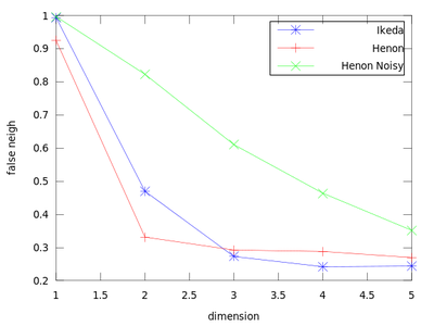
This function uses a method to determine the minimum sufficient embedding dimension. It is based on the False Nearest Neighbors section of the TISEAN documentation. As a demonstration we will create a plot that contains an Ikeda Map, a Henon Map and a Henon Map corrupted by 10% of Gaussian noise.
| Code: Analyzing false nearest neighbors
|
# Create maps
ikd       = ikeda (10000);
hen       = henon (10000);
hen_noisy = hen + std (hen) * 0.02 .* (-6 + sum (rand ([size(hen), 12]), 3));
# Create and plot false nearest neighbors
[dim_ikd, frac_ikd] = false_nearest (ikd(:,1));
[dim_hen, frac_hen] = false_nearest (hen(:,1));
[dim_hen_noisy, frac_hen_noisy] = false_nearest (hen_noisy(:,1));
plot (dim_ikd, frac_ikd, '-b*;Ikeda;',...
      dim_hen, frac_hen, '-r+;Henon;',...
      dim_hen_noisy, frac_hen_noisy, '-gx;Henon Noisy;');
|
The dim_* variables hold the dimension (so here 1:5), and frac_* contain the fraction of false nearest neighbors. From this chart we can obtain the sufficient embedding dimension for each system. For a Henon Map m = 2 is sufficient, but for an Ikeda map it is better to use m = 3.
Finding Unstable Periodic Orbits
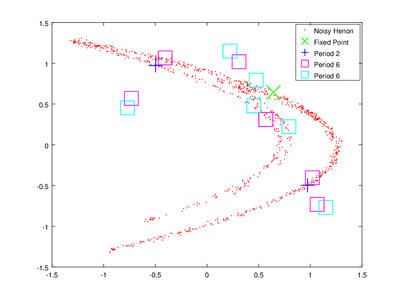
Here I will demonstrate how to find unstable periodic orbits. This section is based on the TISEAN documentation chapter Finding unstable periodic orbits. We will start by finding these orbits using function upo.
| Code: Finding unstable periodic orbits
|
# Create maps
hen             = henon (1000);
hen             = hen + std (hen) * 0.02 .* (-6 + sum (rand ([size(hen), 12]), 3));
# Find orbits
[lengths, data] = upo(hen(:,1), 2, 'p',6,'v',0.1, 'n', 100);
|
The vector lengths contains the size of each of the found orbits and data contains their coordinates. To obtain delay coordinates and plot these orbits onto the original data we will use upoembed.
| Code: Plotting unstable periodic orbits
|
# Create delay coordinates for the orbits and data
up        = upoembed (lengths, data, 1);
delay_hen = delay (hen(:,1));
# Plot all of the data
plot (delay_hen(:,1), delay_hen(:,2), 'r.;Noisy Henon;','markersize',2,...
      up{4}(:,1), up{4}(:,2),'gx;Fixed Point;','markersize',20,'linewidth',1, ...
      up{3}(:,1), up{3}(:,2),'b+;Period 2;','markersize',20,'linewidth',1, ...
      up{2}(:,1), up{2}(:,2),'ms;Period 6;','markersize',20,'linewidth',1, ...
      up{1}(:,1), up{1}(:,2),'cs;Period 6;','markersize',20,'linewidth',1);
|
The plotting options are passed to make the orbits more visible.
Nonlinear Prediction
In this section we will demonstrate some functions from the 'Nonlinear Prediction' chapter of the TISEAN documentation (located here). For now this section will only demonstrate functions that are connected to the Simple Nonlinear Prediction section.
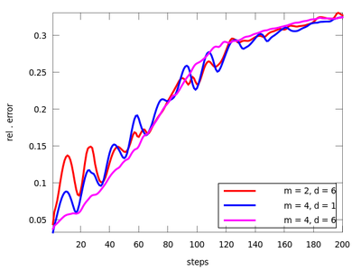
There are three functions in this section: lzo_test, lzo_gm and lzo_run. The first is used to estimate the forecast error for a set of chosen parameters, the second gives some global information about the fit and the third produces predicted points. Let us start with the first one (before starting this example remember to download 'amplitude.dat' from above and start Octave in the directory that contains it). The pairs of parameters (m,d) where chosen after the TISEAN documentation.
| Code: Analyzing forecast errors for various parameters
|
# Load data
load amplitude.dat
# Create different forecast error results
steps = 200;
res1  = lzo_test (amplitude(1:end-200), 'm', 2, 'd', 6, 's', steps);
res2  = lzo_test (amplitude(1:end-200), 'm', 3, 'd', 6, 's', steps);
res3  = lzo_test (amplitude(1:end-200), 'm', 4, 'd', 1, 's', steps);
res4  = lzo_test (amplitude(1:end-200), 'm', 4, 'd', 6, 's', steps);
plot (res1(:,1), res1(:,2), 'r;m = 2, d = 6;', ...
      res2(:,1), res2(:,2), 'g;m = 3, d = 6;',...
      res3(:,1), res3(:,2), 'b;m = 4, d = 1;',...
      res4(:,1), res4(:,2), 'm;m = 4, d = 6;');
|
It seems that the last pair (m = 4, d = 6) is suitable. We will use it to determine the the best neighborhood to use when generating future points.
| Code: Determining the best neighborhood size using lzo_gm
|
gm = lzo_gm (amplitude(1:end-200), 'm', 4, 'd', 6, 's', steps, 'rhigh', 20);
|
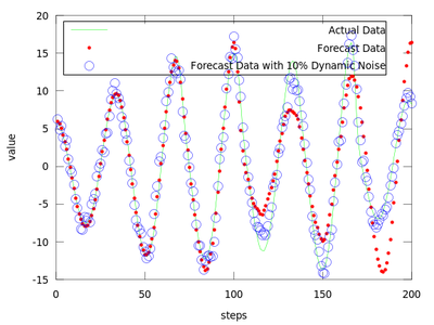
After analyzing gm it is easy to observe that the least error is for the first neighborhood size of gm which is equal to 0.49148. We will use it to produce the prediction vectors. Only the first 4800 datapoints from amplitude are used in order to compare the predicted values with the actual ones for the last 200 points.
| Code: Creating forecast points
|
steps          = 200;
forecast       = lzo_run (amplitude(1:end-200), 'm', 4, 'd', 6, 'r', 0.49148, 'l', steps);
forecast_noisy = lzo_run (amplitude(1:end-200), 'm', 4, 'd', 6, 'r', 0.49148,  ...
                          'dnoise', 10, 'l', steps);
plot (amplitude(end-199:end), 'g;Actual Data;', ...
      forecast, 'r.;Forecast Data;',...
      forecast_noisy, 'bo;Forecast Data with 10% Dynamic Noise;');
|
The difference between finding the proper r and not finding it can be very small.
The produced data is the best local zeroth order fit on the amplitude.dat for (m = 4, d = 6).
Nonlinear Noise Reduction
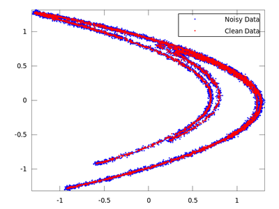
This tutorial show different methods of the 'Nonlinear Noise Reduction' section of the TISEAN documentation (located here). It shows the use of simple nonlinear noise reduction (function lazy) and locally projective nonlinear noise reduction (function ghkss). To start let's create noisy data to work with.
| Code: Creating a noisy henon map
|
hen       = henon (10000);
hen       = hen(:,1); # We only need the first column
hen_noisy = hen + std (hen) * 0.02 .* (-6 + sum (rand ([size(hen), 12]), 3));
|
This created a Henon map contaminated by 2% Gaussian noise à la TISEAN. In the tutorials and exercises on the TISEAN website this would be equivalent to calling makenoise -%2 on the Henon map.
Next we will reduce the noise using simple nonlinear noise reduction lazy.
| Code: Simple nonlinear noise reduction
|
clean       = lazy (hen_noisy,7,-0.06,3);
# Create delay vectors for both the clean and noisy data
delay_clean = delay (clean);
delay_noisy = delay (hen_noisy);
# Plot both on one chart
plot (delay_noisy(:,1), delay_noisy(:,2), 'b.;Noisy Data;','markersize',3,...
      delay_clean(:,1), delay_clean(:,2), 'r.;Clean Data;','markersize',3)
|
On the chart created the red dots represent cleaned up data. It is much closer to the original than the noisy blue set.
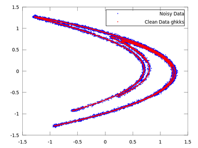
Now we will do the same with ghkss.
| Code: Locally projective nonlinear noise reduction
|
clean = ghkss (hen,'m',7,'q',2,'r',0.05,'k',20,'i',2);
|
The rest of the code is the same as the code used in the lazy example.
Once both results are compared it is quite obvious that for this particular example ghkss is superior to lazy. The TISEAN documentation points out that this is not always the case.
Lyapunov Exponents
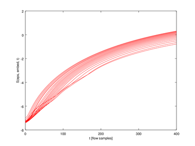
Here I will demonstrate how to use the function lyap_k. It estimates the maximal Lyapunov exponent from a time series (more information available from the TISEAN documentation located here). In this tutorial we will estimate the maximal Lyapunov exponent for various embedding dimensions and then plot them.
| Code: Creating Lyapunov exponents
|
# Create time series
in       = sin((1:2500).'./360) + cos((1:2500).'./180);
# Estimate Lyapunov exponents
mmax_val = 20
lyap_exp = lyap_k (in, 'mmin',2,'mmax',mmax_val,'d',6,'s',400,'t',500);
|
In this function the output (lyap_exp is a 5 x 20 struct array. We will only use one row for the plot.
| Code: Plotting Lyapunov exponents
|
cla reset
hold on
for j=2:mmax_val
  plot (lyap_exp(1,j-1).exp(:,1),lyap_exp(1,j-1).exp(:,2),'r');
endfor
xlabel ("t [flow samples]");
ylabel ("S(eps, embed, t)");
hold off
|
Dimensions and Entropies
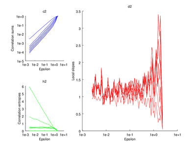
This section is discussed on the TISEAN documentation page. One of the functions discussed is d2. It is used to estimate the correlation sum, correlation dimension and correlation entropy of a time series. The time series used here will be the Henon map.
| Code: Calculation correlation sum, dimension and entropy
|
# Create maps
hen       = henon (10000);
# Calculate the correlation sum, dimension and entropy
vals = d2 (hen, 'd', 1, 'm', 5, 't',50);
# Plot correlation sum
subplot (2,3,1)
do_plot_corr  = @(x) loglog (x{1}(:,1),x{1}(:,2),'b');
hold on
arrayfun (do_plot_corr, {vals.c2});
hold off
xlabel ("Epsilon")
ylabel ("Correlation sums")
title ("c2");
# Plot correlation entropy
subplot (2,3,4)
do_plot_entrop  = @(x) semilogx (x{1}(:,1),x{1}(:,2),'g');
hold on
arrayfun (do_plot_entrop, {vals.h2});
hold off
xlabel ("Epsilon")
ylabel ("Correlation entropies");
title ("h2")
# Plot correlation dimension
subplot (2,3,[2 3 5 6])
do_plot_slope = @(x) semilogx (x{1}(:,1),x{1}(:,2),'r');
hold on
arrayfun (do_plot_slope, {vals.d2});
hold off
xlabel ("Epsilon")
ylabel ("Local slopes")
title ("d2");
|
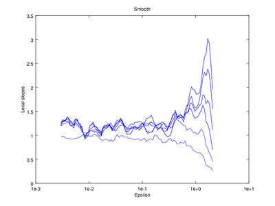
The output of d2 can be further processed using the following functions: av_d2, c2t, c2g. This tutorial will show how to use av_d2 which smooths the output of d2 (usually used to smooth the "d2" field of the output).
| Code: Smooth output of d2
|
# Smooth d2 output
figure 2
smooth = av_d2 (vals,'a',2);
# Plot the smoothed output
do_plot_slope = @(x) semilogx (x{1}(:,1),x{1}(:,2),'b');
hold on
arrayfun (do_plot_slope, {smooth.d2});
hold off
xlabel ("Epsilon")
ylabel ("Local slopes")
title ("Smooth");
|
Optionally the line "figure 2" can be omitted, which will cause the smoothed version to be superimposed on the "raw" version that came straight from d2.
External links
