Bim package: Difference between revisions
No edit summary |
No edit summary |
||
| Line 13: | Line 13: | ||
<math> u(x, y) = u_d(x, y)\qquad \mbox{ on } \Gamma_D </math> | <math> u(x, y) = u_d(x, y)\qquad \mbox{ on } \Gamma_D </math> | ||
<math> -( \varepsilon\ \nabla u(x, y) - \nabla \varphi(x,y)\ u(x, y) ) \cdot \mathbf{n} \qquad \mbox{ on } \Gamma_N</math> | <math> -( \varepsilon\ \nabla u(x, y) - \nabla \varphi(x,y)\ u(x, y) ) \cdot \mathbf{n} = j_N(x, y)\qquad \mbox{ on } \Gamma_N</math> | ||
<b> Create the mesh and precompute the mesh properties </b> | <b> Create the mesh and precompute the mesh properties </b> | ||
To define the geometry of the domain we can use [http://gmsh.geuz.org gmsh]. | |||
the following gmsh input | |||
<pre> | |||
Point (1) = {0, 0, 0, 0.1}; | |||
Point (2) = {1, 1, 0, 0.1}; | |||
Point (3) = {1, 0.9, 0, 0.1}; | |||
Point (4) = {0, 0.1, 0, 0.1}; | |||
Point (5) = {0.3,0.1,-0,0.1}; | |||
Point (6) = {0.4,0.4,-0,0.1}; | |||
Point (7) = {0.5,0.6,0,0.1}; | |||
Point (8) = {0.6,0.9,0,0.1}; | |||
Point (9) = {0.8,0.8,0,0.1}; | |||
Point (10) = {0.2,0.2,-0,0.1}; | |||
Point (11) = {0.3,0.5,0,0.1}; | |||
Point (12) = {0.4,0.7,0,0.1}; | |||
Point (13) = {0.5,1,0,0.1}; | |||
Point (14) = {0.8,0.9,0,0.1}; | |||
Line (1) = {3, 2}; | |||
Line (2) = {4, 1}; | |||
CatmullRom(3) = {1,5,6,7,8,9,3}; | |||
CatmullRom(4) = {4,10,11,12,13,14,2}; | |||
Line Loop(15) = {3,1,-4,2}; | |||
Plane Surface(16) = {15}; | |||
</pre> | |||
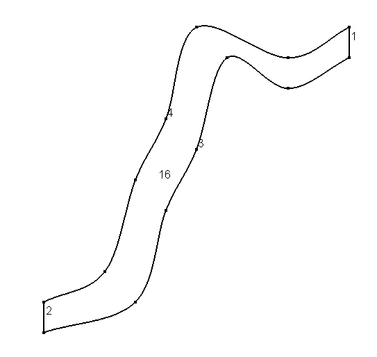
will produce the geometry below | |||
[[File:fiume.png]] | [[File:fiume.png]] | ||
we need to load the mesh into Octave and precompute mesh properties | |||
check out the tutorial for the [[msh_package|msh package]] for info | |||
on the mesh structure | |||
<pre> | <pre> | ||
| Line 27: | Line 59: | ||
</pre> | </pre> | ||
to see the mesh you can use functions from the [fpl] | to see the mesh you can use functions from the [[fpl_package|fpl package]] | ||
<pre> | <pre> | ||
| Line 38: | Line 70: | ||
<b> Construct an initial guess</b> | <b> Construct an initial guess</b> | ||
<b> Set the coefficients for the problem:</b> | |||
Get the node coordinates from the mesh structure | Get the node coordinates from the mesh structure | ||
| Line 49: | Line 79: | ||
</pre> | </pre> | ||
Get the number of elements and nodes in the mesh | Get the number of elements and nodes in the mesh | ||
| Line 65: | Line 89: | ||
<pre> | <pre> | ||
epsilon = .1; | epsilon = .1; | ||
phi = xu+yu; | phi = xu + yu; | ||
</pre> | </pre> | ||
| Line 82: | Line 106: | ||
<pre> | <pre> | ||
GammaD = bim2c_unknowns_on_side(mesh, [1 2]); ## DIRICHLET NODES LIST | |||
GammaN = bim2c_unknowns_on_side(mesh, [3 4]); ## NEUMANN NODES LIST | |||
Corners = setdiff(GammaD,GammaN); | |||
jn = zeros(length(GammaN),1); ## PRESCRIBED NEUMANN FLUXES | |||
ud = 3*xu; ## DIRICHLET DATUM | |||
Ilist = setdiff(1:length(uin),union(Dlist,Nlist)); ## INTERNAL NODES LIST | Ilist = setdiff(1:length(uin),union(Dlist,Nlist)); ## INTERNAL NODES LIST | ||
</pre> | </pre> | ||
Revision as of 21:51, 19 July 2012
This is a short example on how to use bim to solve a DAR problem.
The data for this example can be found in the doc directory inside the
bim installation directory.
We want to solve the equation
with mixed Dirichlet / Neumann boundary conditions
Create the mesh and precompute the mesh properties
To define the geometry of the domain we can use gmsh.
the following gmsh input
Point (1)  = {0, 0, 0, 0.1};
Point (2)  = {1, 1, 0, 0.1};
Point (3)  = {1, 0.9, 0, 0.1};
Point (4)  = {0, 0.1, 0, 0.1};
Point (5) = {0.3,0.1,-0,0.1};
Point (6) = {0.4,0.4,-0,0.1};
Point (7) = {0.5,0.6,0,0.1};
Point (8) = {0.6,0.9,0,0.1};
Point (9) = {0.8,0.8,0,0.1};
Point (10) = {0.2,0.2,-0,0.1};
Point (11) = {0.3,0.5,0,0.1};
Point (12) = {0.4,0.7,0,0.1};
Point (13) = {0.5,1,0,0.1};
Point (14) = {0.8,0.9,0,0.1};

Line (1)  = {3, 2};
Line (2) = {4, 1};

CatmullRom(3) = {1,5,6,7,8,9,3};
CatmullRom(4) = {4,10,11,12,13,14,2};
Line Loop(15) = {3,1,-4,2};
Plane Surface(16) = {15};
will produce the geometry below
we need to load the mesh into Octave and precompute mesh properties check out the tutorial for the msh package for info on the mesh structure
[mesh] = msh2m_gmsh("fiume","scale",1,"clscale",.1);
[mesh] = bim2c_mesh_properties(mesh);
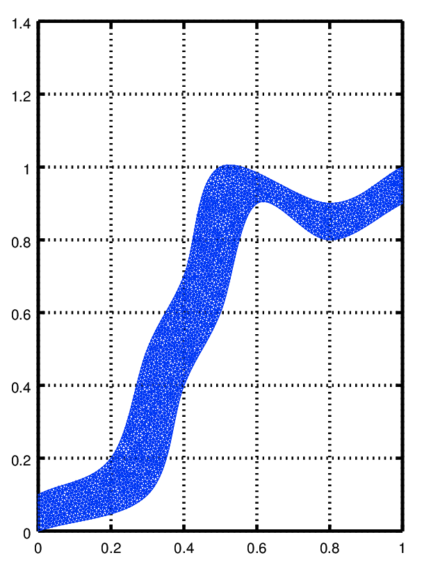
to see the mesh you can use functions from the fpl package
pdemesh (mesh.p, mesh.e, mesh.t)
view (2)
Construct an initial guess
Set the coefficients for the problem:
Get the node coordinates from the mesh structure
xu     = mesh.p(1,:).';
yu     = mesh.p(2,:).';
Get the number of elements and nodes in the mesh
nelems = columns(mesh.t);
nnodes = columns(mesh.p);
epsilon = .1;
phi     = xu + yu;
Construct the discretized operators
AdvDiff = bim2a_advection_diffusion(mesh, epsilon, 1, phi);
Mass    = bim2a_reaction(mesh,delta,zeta);
b       = bim2a_rhs(mesh,f,g);
A       = AdvDiff + Mass;
To Apply Boundary Conditions, partition LHS and RHS
The tags of the sides are assigned by gmsh
GammaD = bim2c_unknowns_on_side(mesh, [1 2]); 	   ## DIRICHLET NODES LIST
GammaN = bim2c_unknowns_on_side(mesh, [3 4]); 	   ## NEUMANN NODES LIST
Corners = setdiff(GammaD,GammaN);
jn    = zeros(length(GammaN),1);           	   ## PRESCRIBED NEUMANN FLUXES
ud    = 3*xu;                                      ## DIRICHLET DATUM
Ilist = setdiff(1:length(uin),union(Dlist,Nlist)); ## INTERNAL NODES LIST
Add = A(Dlist,Dlist);
Adn = A(Dlist,Nlist); ## shoud be all zeros hopefully!!
Adi = A(Dlist,Ilist);

And = A(Nlist,Dlist); ## shoud be all zeros hopefully!!
Ann = A(Nlist,Nlist);
Ani = A(Nlist,Ilist);

Aid = A(Ilist,Dlist);
Ain = A(Ilist,Nlist);
Aii = A(Ilist,Ilist);

bd = b(Dlist);
bn = b(Nlist);
bi = b(Ilist);

ud = uin(Dlist);
un = uin(Nlist);
ui = uin(Ilist);
Solve for the displacements
temp = [Ann Ani ; Ain Aii ] \ [ Fn+bn-And*ud ; bi-Aid*ud];
un   = temp(1:length(un));
ui   = temp(length(un)+1:end);
u(Dlist) = ud;
u(Ilist) = ui;
u(Nlist) = un;
Compute the fluxes through Dirichlet sides
Fd = Add * ud + Adi * ui + Adn*un - bd;
Compute the gradient of the solution
[gx, gy] = bim2c_pde_gradient(mesh,u);
Compute the internal Advection-Diffusion flux
[jxglob,jyglob] = bim2c_global_flux(mesh,u,alfa,gamma,eta,beta);
Save data for later visualization
fpl_dx_write_field("dxdata",mesh,[gx; gy]',"Gradient",1,2,1);
fpl_vtk_write_field ("vtkdata", mesh, {}, {[gx; gy]', "Gradient"}, 1);


