Bim package: Difference between revisions
No edit summary |
m (Unified layout. Links https.) |
||
| (32 intermediate revisions by 6 users not shown) | |||
| Line 1: | Line 1: | ||
The {{Forge|bim}} package is part of the [[Octave Forge]] project. It is a package for solving Diffusion Advection Reaction (DAR) Partial Differential Equations based on the Finite Volume Scharfetter-Gummel (FVSG) method a.k.a Box Integration Method (BIM). | |||
== Tutorials == | |||
=== 2D Diffusion Advection Reaction example === | |||
The | This is a short example on how to use <tt>bim</tt> to solve a 2D Diffusion Advection Reaction problem. | ||
<!-- The complete code for this example is on [[Agora]] at this [http://agora.octave.org/snippet/1bqV link] -->. | |||
We want to solve the equation | We want to solve the equation | ||
<math> -\mathrm{div}\ ( \varepsilon\ \nabla u(x, y) - \nabla \varphi(x,y)\ u(x, y) ) ) + u(x, y) = 1 \qquad in \Omega</math> | <math> -\mathrm{div}\ ( \varepsilon\ \nabla u(x, y) - \nabla \varphi(x,y)\ u(x, y) ) ) + u(x, y) = 1 \qquad \mbox{ in } \Omega</math> | ||
<math> \varphi(x, y)\ =\ x + y </math> | <math> \varphi(x, y)\ =\ x + y </math> | ||
| Line 54: | Line 58: | ||
on the mesh structure | on the mesh structure | ||
< | {{Code|Meshing the 2D problem|<syntaxhighlight lang="octave" style="font-size:13px"> | ||
[mesh] = msh2m_gmsh ("fiume","scale",1,"clscale",.1); | [mesh] = msh2m_gmsh ("fiume","scale",1,"clscale",.1); | ||
[mesh] = bim2c_mesh_properties (mesh); | [mesh] = bim2c_mesh_properties (mesh); | ||
</ | </syntaxhighlight>}} | ||
to see the mesh you can use functions from the [[fpl_package|fpl package]] | to see the mesh you can use functions from the [[fpl_package|fpl package]] | ||
< | {{Code|Visualizing the mesh for the 2D problem|<syntaxhighlight lang="octave" style="font-size:13px"> | ||
pdemesh (mesh.p, mesh.e, mesh.t) | pdemesh (mesh.p, mesh.e, mesh.t) | ||
view (2) | view (2) | ||
</ | </syntaxhighlight>}} | ||
[[File:fiume_msh.png]] | [[File:fiume_msh.png]] | ||
| Line 73: | Line 77: | ||
Get the node coordinates from the mesh structure | Get the node coordinates from the mesh structure | ||
< | {{Code|Get mesh coordinates in the 2D problem|<syntaxhighlight lang="octave" style="font-size:13px"> | ||
xu = mesh.p(1,:).'; | xu = mesh.p(1,:).'; | ||
yu = mesh.p(2,:).'; | yu = mesh.p(2,:).'; | ||
</ | </syntaxhighlight> | ||
}} | |||
Get the number of elements and nodes in the mesh | Get the number of elements and nodes in the mesh | ||
< | {{Code|Get number of elements in the 2D problem|<syntaxhighlight lang="octave" style="font-size:13px"> | ||
nelems = columns (mesh.t); | nelems = columns (mesh.t); | ||
nnodes = columns (mesh.p); | nnodes = columns (mesh.p); | ||
</ | </syntaxhighlight>}} | ||
< | {{Code|Set value of coefficients for the 2D problem|<syntaxhighlight lang="octave" style="font-size:13px"> | ||
epsilon = .1; | epsilon = .1; | ||
phi = xu + yu; | phi = xu + yu; | ||
</ | </syntaxhighlight>}} | ||
<b> Construct the discretized operators</b> | <b> Construct the discretized operators</b> | ||
< | {{Code|Discretized operators for the 2D problem|<syntaxhighlight lang="octave" style="font-size:13px"> | ||
AdvDiff = bim2a_advection_diffusion (mesh, epsilon, 1, 1, phi); | AdvDiff = bim2a_advection_diffusion (mesh, epsilon, 1, 1, phi); | ||
Mass = bim2a_reaction (mesh, 1, 1); | Mass = bim2a_reaction (mesh, 1, 1); | ||
b = bim2a_rhs (mesh,f,g); | b = bim2a_rhs (mesh,f,g); | ||
A = AdvDiff + Mass; | A = AdvDiff + Mass; | ||
</ | </syntaxhighlight>}} | ||
<b> To Apply Boundary Conditions, partition LHS and RHS</b> | <b> To Apply Boundary Conditions, partition LHS and RHS</b> | ||
| Line 105: | Line 110: | ||
and <math> \Gamma_D </math> be the rest of the boundary | and <math> \Gamma_D </math> be the rest of the boundary | ||
< | {{Code|Boundary conditions for the 2D problem|<syntaxhighlight lang="octave" style="font-size:13px"> | ||
GammaD = bim2c_unknowns_on_side (mesh, [1 2]); ## DIRICHLET NODES LIST | GammaD = bim2c_unknowns_on_side (mesh, [1 2]); ## DIRICHLET NODES LIST | ||
GammaN = bim2c_unknowns_on_side (mesh, [3 4]); ## NEUMANN NODES LIST | GammaN = bim2c_unknowns_on_side (mesh, [3 4]); ## NEUMANN NODES LIST | ||
| Line 113: | Line 118: | ||
ud = 3*xu; ## DIRICHLET DATUM | ud = 3*xu; ## DIRICHLET DATUM | ||
Omega = setdiff (1:nnodes, union (GammaD, GammaN)); ## INTERIOR NODES LIST | Omega = setdiff (1:nnodes, union (GammaD, GammaN)); ## INTERIOR NODES LIST | ||
Add = A(GammaD, GammaD); | Add = A(GammaD, GammaD); | ||
Adn = A(GammaD, GammaN); ## shoud be all zeros hopefully!! | Adn = A(GammaD, GammaN); ## shoud be all zeros hopefully!! | ||
| Line 132: | Line 134: | ||
bn = b(GammaN); | bn = b(GammaN); | ||
bi = b(Omega); | bi = b(Omega); | ||
</ | </syntaxhighlight>}} | ||
<B> Solve for the | <B> Solve for the tracer density</B> | ||
< | {{Code|Compute solution of the 2D problem|<syntaxhighlight lang="octave" style="font-size:13px"> | ||
temp = [Ann Ani ; Ain Aii ] \ [ jn+bn-And*ud(GammaD) ; bi-Aid*ud(GammaD)]; | temp = [Ann Ani ; Ain Aii ] \ [ jn+bn-And*ud(GammaD) ; bi-Aid*ud(GammaD)]; | ||
u = ud; | u = ud; | ||
u(GammaN) = temp(1:numel (GammaN)); | u(GammaN) = temp(1:numel (GammaN)); | ||
u(Omega) = temp(length(GammaN)+1:end); | u(Omega) = temp(length(GammaN)+1:end); | ||
</ | </syntaxhighlight>}} | ||
<b> Compute the fluxes through Dirichlet sides</b><br> | <b> Compute the fluxes through Dirichlet sides</b><br> | ||
< | {{Code|Boundary fluxes in the 2D problem|<syntaxhighlight lang="octave" style="font-size:13px"> | ||
jd = [Add Adi Adn] * u([GammaD; Omega; GammaN]) - bd; | jd = [Add Adi Adn] * u([GammaD; Omega; GammaN]) - bd; | ||
</ | </syntaxhighlight>}} | ||
<B> Compute the gradient of the solution </B> | <B> Compute the gradient of the solution </B> | ||
< | {{Code|Gradient of solution in the 2D problem|<syntaxhighlight lang="octave" style="font-size:13px"> | ||
[gx, gy] = bim2c_pde_gradient (mesh, u); | [gx, gy] = bim2c_pde_gradient (mesh, u); | ||
</ | </syntaxhighlight>}} | ||
<B> Compute the internal Advection-Diffusion flux</B> | <B> Compute the internal Advection-Diffusion flux</B> | ||
< | {{Code|Total flux for the 2D problem|<syntaxhighlight lang="octave" style="font-size:13px"> | ||
[jxglob, jyglob] = bim2c_global_flux (mesh, u, epsilon*ones(nelems, 1), ones(nnodes, 1), ones(nnodes, 1), phi); | [jxglob, jyglob] = bim2c_global_flux (mesh, u, epsilon*ones(nelems, 1), ones(nnodes, 1), ones(nnodes, 1), phi); | ||
</ | </syntaxhighlight>}} | ||
<B> Export data to VTK format</B> | <B> Export data to VTK format</B> | ||
| Line 167: | Line 170: | ||
or [[https://wci.llnl.gov/codes/visit/|visit]] | or [[https://wci.llnl.gov/codes/visit/|visit]] | ||
< | {{Code|Export the solution of the 2D problem to vtk|<syntaxhighlight lang="octave" style="font-size:13px"> | ||
fpl_vtk_write_field ("vtkdata", mesh, {u, "Solution"}, {[gx; gy]', "Gradient"}, 1); | fpl_vtk_write_field ("vtkdata", mesh, {u, "Solution"}, {[gx; gy]', "Gradient"}, 1); | ||
</ | </syntaxhighlight>}} | ||
you can also plot your data directly in Octave using <code> pdesurf </code> | you can also plot your data directly in Octave using <code> pdesurf </code> | ||
< | {{Code|Rubbersheet visualization of the solution of the 2D problem|<syntaxhighlight lang="octave" style="font-size:13px"> | ||
pdesurf (mesh.p, mesh.t, u) | pdesurf (mesh.p, mesh.t, u) | ||
</ | </syntaxhighlight>}} | ||
it will look like this | it will look like this | ||
| Line 181: | Line 184: | ||
[[File:fiume_sol_pdesurf.png|500px]] | [[File:fiume_sol_pdesurf.png|500px]] | ||
[[ | === 3D Time dependent problem === | ||
[[Category: | |||
Here is an example of a 3D time-dependent Advection-Diffusion equation that uses <code> lsode </code> for time-stepping. | |||
The equation being solved is | |||
<math> \frac{\partial u}{\partial t} - \mathrm{div } \left(.01 \nabla u - u \nabla \varphi \right) | |||
= 0 \qquad \mbox{ in } \Omega \times [0, T] =[0, 1]^3 \times [0, 1] </math> | |||
<math> ~\varphi = x + y - z </math> | |||
<math> - \left(.01 \nabla u - u \nabla \varphi \right) \cdot \mathbf{n} = 0 | |||
\qquad \mbox{ on } \partial \Omega</math> | |||
The initial condition is | |||
<math> u = \exp (- \left(\frac{x-.2}{.2}\right)^2 - \left(\frac{y-.2}{.2}\right)^2 - \left(\frac{z-.2}{.2}\right)^2)</math> | |||
{{Code|Define the 3D problem|<syntaxhighlight lang="octave" style="font-size:13px"> | |||
pkg load bim | |||
x = linspace (0, 1, 40); | |||
y = z = linspace (0, 1, 20); | |||
msh = bim3c_mesh_properties (msh3m_structured_mesh (x, y, z, 1, 1:6)); | |||
nn = columns (msh.p); | |||
ne = columns (msh.t); | |||
x = msh.p(1, :).'; | |||
y = msh.p(2, :).'; | |||
z = msh.p(3, :).'; | |||
x0 = .2; sx = .1; | |||
y0 = .2; sy = .1; | |||
z0 = .8; sz = .1; | |||
u = exp (- ((x-x0)/(2*sx)) .^2 - ((y-y0)/(2*sy)) .^2 - ((z-z0)/(2*sz)) .^2); | |||
A = bim3a_advection_diffusion (msh, .01*ones(ne, 1), 100*(x+y-z)); | |||
M = bim3a_reaction (msh, 1, 1); | |||
function du = f (u, t, A, M) | |||
du = - M \ (A * u); | |||
endfunction | |||
time = linspace (0, 1, 30); | |||
lsode_options ("integration method", "adams"); | |||
U = lsode (@(u, t) f(u, t, A, M), u, time); | |||
for ii = 1:1:numel (time) | |||
name = sprintf ("u_%3.3d", ii); | |||
delete ([name ".vtu"]); | |||
fpl_vtk_write_field (name, msh, {U(ii,:)', 'u'}, {}, 1); | |||
endfor | |||
</syntaxhighlight>}} | |||
[http://youtu.be/2E6Z_AcV8CQ This is a video] showing the .3 isosurface of the solution. | |||
== External links == | |||
* [https://octave.sourceforge.io/bim/index.html BIM package at Octave Forge]. | |||
== Scientific papers using BIM == | |||
* [https://doi.org/10.1016/j.jcp.2004.10.029 de Falco, C., Gatti, E., Lacaita, A. L., & Sacco, R. (2005). Quantum-corrected drift-diffusion models for transport in semiconductor devices. Journal of Computational Physics, 204(2), 533-561.] | |||
* [https://doi.org/10.1016/j.jcp.2008.11.010 de Falco, C., Jerome, J.W. and Sacco, R., 2009. Quantum-corrected drift-diffusion models: Solution fixed point map and finite element approximation. Journal of Computational Physics, 228(5), pp.1770-1789.] | |||
* [http://www.math.ualberta.ca/ijnam/Volume-7-2010/No-3-10/2010-03-04.pdf de Falco, C. and O'riordan, E., 2010. INTERIOR LAYERS IN A REACTION DIFFUSION EQUATION WITH A DISCONTINUOUS DIFFUSION COEFFICIENT. International Journal of Numerical Analysis & Modeling, 7(3).] | |||
* [https://doi.org/10.1016/j.cma.2010.01.018 de Falco, C., Sacco, R. and Verri, M., 2010. Analytical and numerical study of photocurrent transients in organic polymer solar cells. Computer Methods in Applied Mechanics and Engineering, 199(25), pp.1722-1732.] | |||
* [https://doi.org/10.1016/j.cma.2012.06.018 de Falco, C., Porro, M., Sacco, R. and Verri, M., 2012. Multiscale modeling and simulation of organic solar cells. Computer Methods in Applied Mechanics and Engineering, 245, pp.102-116.] | |||
* [http://link.springer.com/chapter/10.1007/978-3-540-71980-9_5 de Falco, C., Denk, G. and Schultz, R., 2007. A demonstrator platform for coupled multiscale simulation. In Scientific Computing in Electrical Engineering (pp. 63-71). Springer Berlin Heidelberg.] | |||
* [https://doi.org/10.1016/j.orgel.2014.12.001 Maddalena, F., de Falco, C., Caironi, M. and Natali, D., 2015. Assessing the width of Gaussian density of states in organic semiconductors. Organic Electronics, 17, pp.304-318.] | |||
* [http://link.springer.com/chapter/10.1007/978-3-642-12294-1_35 Alì, G., Bartel, A., Culpo, M. and de Falco, C., 2010. Analysis of a PDE thermal element model for electrothermal circuit simulation. In Scientific Computing in Electrical Engineering SCEE 2008 (pp. 273-280). Springer Berlin Heidelberg.] | |||
* [http://onlinelibrary.wiley.com/doi/10.1002/pamm.200810065/full Culpo, M. and De Falco, C., 2008. Dynamical iteration schemes for coupled simulation in nanoelectronics. PAMM, 8(1), pp.10065-10068.] | |||
* [https://doi.org/10.1108/COMPEL-12-2012-0365 Porro, M., de Falco, C., Verri, M., Lanzani, G. and Sacco, R., 2014. Multiscale simulation of organic heterojunction light harvesting devices. COMPEL: The International Journal for Computation and Mathematics in Electrical and Electronic Engineering, 33(4), pp.1107-1122.] | |||
* [http://dx.doi.org/10.1063/1.4709483 Ciucci, F., de Falco, C., Guzman, M.I., Lee, S. and Honda, T., 2012. Chemisorption on semiconductors: The role of quantum corrections on the space charge regions in multiple dimensions. Applied Physics Letters, 100(18), p.183106.] | |||
* [https://link.springer.com/chapter/10.1007%2F978-3-642-12294-1_36 Culpo, M., de Falco, C., Denk, G. and Voigtmann, S., 2010. Automatic thermal network extraction and multiscale electro-thermal simulation. In Scientific Computing in Electrical Engineering SCEE 2008 (pp. 281-288). Springer Berlin Heidelberg.] | |||
* [https://link.springer.com/chapter/10.1007/978-3-642-12110-4_33 Culpo, M., de Falco, C. and O’Riordan, E., 2010. Patches of finite elements for singularly-perturbed diffusion reaction equations with discontinuous coefficients. In Progress in Industrial Mathematics at ECMI 2008 (pp. 235-240). Springer Berlin Heidelberg.] | |||
[[Category:Octave Forge]] | |||
Latest revision as of 09:53, 14 June 2019
The bim package is part of the Octave Forge project. It is a package for solving Diffusion Advection Reaction (DAR) Partial Differential Equations based on the Finite Volume Scharfetter-Gummel (FVSG) method a.k.a Box Integration Method (BIM).
Tutorials[edit]
2D Diffusion Advection Reaction example[edit]
This is a short example on how to use bim to solve a 2D Diffusion Advection Reaction problem. .
We want to solve the equation
with mixed Dirichlet / Neumann boundary conditions
Create the mesh and precompute the mesh properties
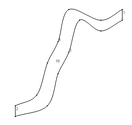
To define the geometry of the domain we can use gmsh.
the following gmsh input
Point (1)  = {0, 0, 0, 0.1};
Point (2)  = {1, 1, 0, 0.1};
Point (3)  = {1, 0.9, 0, 0.1};
Point (4)  = {0, 0.1, 0, 0.1};
Point (5) = {0.3,0.1,-0,0.1};
Point (6) = {0.4,0.4,-0,0.1};
Point (7) = {0.5,0.6,0,0.1};
Point (8) = {0.6,0.9,0,0.1};
Point (9) = {0.8,0.8,0,0.1};
Point (10) = {0.2,0.2,-0,0.1};
Point (11) = {0.3,0.5,0,0.1};
Point (12) = {0.4,0.7,0,0.1};
Point (13) = {0.5,1,0,0.1};
Point (14) = {0.8,0.9,0,0.1};

Line (1)  = {3, 2};
Line (2) = {4, 1};

CatmullRom(3) = {1,5,6,7,8,9,3};
CatmullRom(4) = {4,10,11,12,13,14,2};
Line Loop(15) = {3,1,-4,2};
Plane Surface(16) = {15};
will produce the geometry below
we need to load the mesh into Octave and precompute mesh properties check out the tutorial for the msh package for info on the mesh structure
| Code: Meshing the 2D problem |
[mesh] = msh2m_gmsh ("fiume","scale",1,"clscale",.1);
[mesh] = bim2c_mesh_properties (mesh);
|
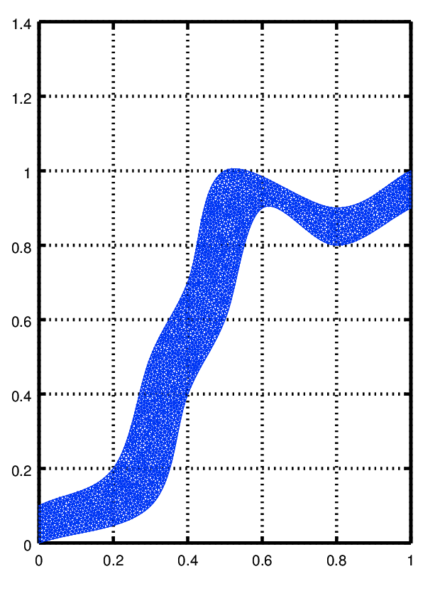
to see the mesh you can use functions from the fpl package
| Code: Visualizing the mesh for the 2D problem |
pdemesh (mesh.p, mesh.e, mesh.t)
view (2)
|
Set the coefficients for the problem:
Get the node coordinates from the mesh structure
| Code: Get mesh coordinates in the 2D problem |
xu     = mesh.p(1,:).';
yu     = mesh.p(2,:).';
|
Get the number of elements and nodes in the mesh
| Code: Get number of elements in the 2D problem |
nelems = columns (mesh.t);
nnodes = columns (mesh.p);
|
| Code: Set value of coefficients for the 2D problem |
epsilon = .1;
phi     = xu + yu;
|
Construct the discretized operators
| Code: Discretized operators for the 2D problem |
AdvDiff = bim2a_advection_diffusion (mesh, epsilon, 1, 1, phi);
Mass    = bim2a_reaction (mesh, 1, 1);
b       = bim2a_rhs (mesh,f,g);
A       = AdvDiff + Mass;
|
To Apply Boundary Conditions, partition LHS and RHS
The tags of the sides are assigned by gmsh we let be composed by sides 1 and 2 and be the rest of the boundary
| Code: Boundary conditions for the 2D problem |
GammaD = bim2c_unknowns_on_side (mesh, [1 2]); 	    ## DIRICHLET NODES LIST
GammaN = bim2c_unknowns_on_side (mesh, [3 4]); 	    ## NEUMANN NODES LIST
GammaN = setdiff (GammaN, GammaD);

jn    = zeros (length (GammaN),1);           	    ## PRESCRIBED NEUMANN FLUXES
ud    = 3*xu;                                       ## DIRICHLET DATUM
Omega = setdiff (1:nnodes, union (GammaD, GammaN)); ## INTERIOR NODES LIST

Add = A(GammaD, GammaD);
Adn = A(GammaD, GammaN); ## shoud be all zeros hopefully!!
Adi = A(GammaD, Omega);

And = A(GammaN, GammaD); ## shoud be all zeros hopefully!!
Ann = A(GammaN, GammaN);
Ani = A(GammaN, Omega);

Aid = A(Omega, GammaD);
Ain = A(Omega, GammaN);
Aii = A(Omega, Omega);

bd = b(GammaD);
bn = b(GammaN);
bi = b(Omega);
|
Solve for the tracer density
| Code: Compute solution of the 2D problem |
temp = [Ann Ani ; Ain Aii ] \ [ jn+bn-And*ud(GammaD) ; bi-Aid*ud(GammaD)];
u = ud;
u(GammaN)  = temp(1:numel (GammaN));
u(Omega)   = temp(length(GammaN)+1:end);
|
Compute the fluxes through Dirichlet sides
| Code: Boundary fluxes in the 2D problem |
jd = [Add Adi Adn] * u([GammaD; Omega; GammaN]) - bd;
|
Compute the gradient of the solution
| Code: Gradient of solution in the 2D problem |
[gx, gy] = bim2c_pde_gradient (mesh, u);
|
Compute the internal Advection-Diffusion flux
| Code: Total flux for the 2D problem |
[jxglob, jyglob] = bim2c_global_flux (mesh, u, epsilon*ones(nelems, 1), ones(nnodes, 1), ones(nnodes, 1), phi);
|
Export data to VTK format
The resut can be exported to vtk format to visualize with [[1]] or [[2]]
| Code: Export the solution of the 2D problem to vtk |
fpl_vtk_write_field ("vtkdata", mesh, {u, "Solution"}, {[gx; gy]', "Gradient"}, 1);
|
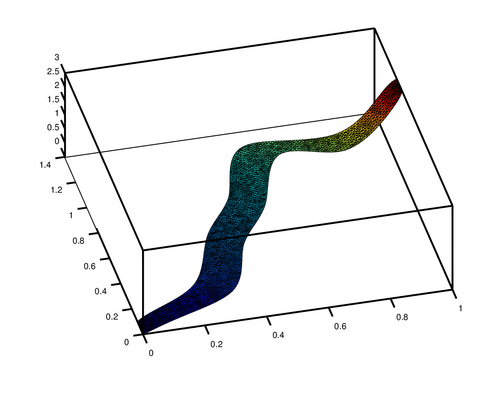
you can also plot your data directly in Octave using pdesurf
| Code: Rubbersheet visualization of the solution of the 2D problem |
pdesurf (mesh.p, mesh.t, u)
|
it will look like this
3D Time dependent problem[edit]
Here is an example of a 3D time-dependent Advection-Diffusion equation that uses lsode for time-stepping.
The equation being solved is
The initial condition is
| Code: Define the 3D problem |
pkg load bim

x = linspace (0, 1, 40);
y = z = linspace (0, 1, 20);
msh = bim3c_mesh_properties (msh3m_structured_mesh (x, y, z, 1, 1:6));
nn = columns (msh.p);
ne = columns (msh.t);

x = msh.p(1, :).';
y = msh.p(2, :).';
z = msh.p(3, :).';

x0 = .2; sx = .1;
y0 = .2; sy = .1;
z0 = .8; sz = .1;

u = exp (- ((x-x0)/(2*sx)) .^2 - ((y-y0)/(2*sy)) .^2 - ((z-z0)/(2*sz)) .^2);

A = bim3a_advection_diffusion (msh, .01*ones(ne, 1), 100*(x+y-z));
M = bim3a_reaction (msh, 1, 1);

function du = f (u, t, A, M)
  du = - M \ (A * u);
endfunction

time = linspace (0, 1, 30);
lsode_options ("integration method", "adams");
U = lsode (@(u, t) f(u, t, A, M), u, time);

for ii = 1:1:numel (time)
  name = sprintf ("u_%3.3d", ii);
  delete ([name ".vtu"]);
  fpl_vtk_write_field (name, msh, {U(ii,:)', 'u'}, {}, 1);
endfor
|
This is a video showing the .3 isosurface of the solution.
External links[edit]


![{\displaystyle {\frac {\partial u}{\partial t}}-\mathrm {div} \left(.01\nabla u-u\nabla \varphi \right)=0\qquad {\mbox{ in }}\Omega \times [0,T]=[0,1]^{3}\times [0,1]}](https://wikimedia.org/api/rest_v1/media/math/render/svg/3733151631f4fa649cf6dc34c0433c240f6a9c08)


